What kind of movie should I direct? :)
Publish date: Sep 4, 2021Tags: R data analytics data visualization movie
Analysis of movies - IMDB dataset
We will look at a subset sample of movies, taken from the Kaggle IMDB 5000 movie dataset
Besides the obvious variables of title, genre, director, year, and duration, the rest of the variables are as follows:
gross: The gross earnings in the US box office, not adjusted for inflationbudget: The movie’s budgetcast_facebook_likes: the number of facebook likes cast members receivedvotes: the number of people who voted for (or rated) the movie in IMDBreviews: the number of reviews for that movierating: IMDB average rating
Import, inspection, and cleaning of dataset-
From the dataset, we can see that: 1. There are no missing values in the dataset. 2. The movies with duplicated entries. There are Duplicates (2907 distinct titles in 2961 rows) The following piece of code shows how we have cleaned it.
movies <- read_csv(here::here("data", "movies.csv"))
glimpse(movies)
## Rows: 2,961
## Columns: 11
## $ title <chr> "Avatar", "Titanic", "Jurassic World", "The Avenge…
## $ genre <chr> "Action", "Drama", "Action", "Action", "Action", "…
## $ director <chr> "James Cameron", "James Cameron", "Colin Trevorrow…
## $ year <dbl> 2009, 1997, 2015, 2012, 2008, 1999, 1977, 2015, 20…
## $ duration <dbl> 178, 194, 124, 173, 152, 136, 125, 141, 164, 93, 1…
## $ gross <dbl> 760505847, 658672302, 652177271, 623279547, 533316…
## $ budget <dbl> 2.37e+08, 2.00e+08, 1.50e+08, 2.20e+08, 1.85e+08, …
## $ cast_facebook_likes <dbl> 4834, 45223, 8458, 87697, 57802, 37723, 13485, 920…
## $ votes <dbl> 886204, 793059, 418214, 995415, 1676169, 534658, 9…
## $ reviews <dbl> 3777, 2843, 1934, 2425, 5312, 3917, 1752, 1752, 35…
## $ rating <dbl> 7.9, 7.7, 7.0, 8.1, 9.0, 6.5, 8.7, 7.5, 8.5, 7.2, …# no missing values. There are Duplicates (2907 distinct titles in 2961 rows).
skim(movies)| Name | movies |
| Number of rows | 2961 |
| Number of columns | 11 |
| _______________________ | |
| Column type frequency: | |
| character | 3 |
| numeric | 8 |
| ________________________ | |
| Group variables | None |
Variable type: character
| skim_variable | n_missing | complete_rate | min | max | empty | n_unique | whitespace |
|---|---|---|---|---|---|---|---|
| title | 0 | 1 | 1 | 83 | 0 | 2907 | 0 |
| genre | 0 | 1 | 5 | 11 | 0 | 17 | 0 |
| director | 0 | 1 | 3 | 32 | 0 | 1366 | 0 |
Variable type: numeric
| skim_variable | n_missing | complete_rate | mean | sd | p0 | p25 | p50 | p75 | p100 | hist |
|---|---|---|---|---|---|---|---|---|---|---|
| year | 0 | 1 | 2002.90 | 9.95 | 1920.0 | 1999.0 | 2004.0 | 2010.0 | 2016.0 | ▁▁▁▂▇ |
| duration | 0 | 1 | 109.65 | 22.17 | 37.0 | 95.0 | 106.0 | 119.0 | 330.0 | ▃▇▁▁▁ |
| gross | 0 | 1 | 58090400.90 | 72469621.94 | 703.0 | 12276810.0 | 34703228.0 | 75590286.0 | 760505847.0 | ▇▁▁▁▁ |
| budget | 0 | 1 | 40619384.06 | 43682007.78 | 218.0 | 11000000.0 | 26000000.0 | 55000000.0 | 300000000.0 | ▇▂▁▁▁ |
| cast_facebook_likes | 0 | 1 | 12393.76 | 20530.11 | 0.0 | 2241.0 | 4604.0 | 16926.0 | 656730.0 | ▇▁▁▁▁ |
| votes | 0 | 1 | 109307.49 | 158143.91 | 5.0 | 19918.0 | 55749.0 | 133348.0 | 1689764.0 | ▇▁▁▁▁ |
| reviews | 0 | 1 | 503.31 | 493.74 | 2.0 | 199.0 | 364.0 | 631.0 | 5312.0 | ▇▁▁▁▁ |
| rating | 0 | 1 | 6.39 | 1.05 | 1.6 | 5.8 | 6.5 | 7.1 | 9.3 | ▁▁▆▇▁ |
# show the duplicate movies
movies %>% count(title, sort=T)
## # A tibble: 2,907 × 2
## title n
## <chr> <int>
## 1 Home 3
## 2 A Nightmare on Elm Street 2
## 3 Across the Universe 2
## 4 Alice in Wonderland 2
## 5 Aloha 2
## 6 Around the World in 80 Days 2
## 7 Brothers 2
## 8 Carrie 2
## 9 Chasing Liberty 2
## 10 Cinderella 2
## # … with 2,897 more rows# to see what happens with the duplicates
movies %>% filter(title=="Homes")## # A tibble: 0 × 11
## # … with 11 variables: title <chr>, genre <chr>, director <chr>, year <dbl>,
## # duration <dbl>, gross <dbl>, budget <dbl>, cast_facebook_likes <dbl>,
## # votes <dbl>, reviews <dbl>, rating <dbl># `distinct` function can only keep the first entry but not latest
# movies <- distinct(movies, title, .keep_all=T)
length(unique(movies$title))## [1] 2907movies <- movies %>%
group_by(title) %>%
filter(votes == max(votes)) %>%
ungroup()
# there are still duplicates
movies %>% count(title, sort=T)## # A tibble: 2,907 × 2
## title n
## <chr> <int>
## 1 Chasing Liberty 2
## 2 10 Cloverfield Lane 1
## 3 10 Days in a Madhouse 1
## 4 10 Things I Hate About You 1
## 5 102 Dalmatians 1
## 6 10th & Wolf 1
## 7 12 Rounds 1
## 8 12 Years a Slave 1
## 9 127 Hours 1
## 10 13 Going on 30 1
## # … with 2,897 more rows# to see what happens with the duplicates
movies %>% filter(title=="Chasing Liberty")## # A tibble: 2 × 11
## title genre director year duration gross budget cast_facebook_l… votes
## <chr> <chr> <chr> <dbl> <dbl> <dbl> <dbl> <dbl> <dbl>
## 1 Chasing… Comedy Andy Cad… 2004 101 1.22e7 2.3e7 842 30092
## 2 Chasing… Comedy Andy Cad… 2004 101 1.22e7 2.3e7 829 30092
## # … with 2 more variables: reviews <dbl>, rating <dbl># do the filter only for the entries of Chasing Liberty
movies <- movies %>%
group_by(title) %>%
filter(cast_facebook_likes==max(cast_facebook_likes)) %>%
ungroup()
skim(movies)| Name | movies |
| Number of rows | 2907 |
| Number of columns | 11 |
| _______________________ | |
| Column type frequency: | |
| character | 3 |
| numeric | 8 |
| ________________________ | |
| Group variables | None |
Variable type: character
| skim_variable | n_missing | complete_rate | min | max | empty | n_unique | whitespace |
|---|---|---|---|---|---|---|---|
| title | 0 | 1 | 1 | 83 | 0 | 2907 | 0 |
| genre | 0 | 1 | 5 | 11 | 0 | 17 | 0 |
| director | 0 | 1 | 3 | 32 | 0 | 1366 | 0 |
Variable type: numeric
| skim_variable | n_missing | complete_rate | mean | sd | p0 | p25 | p50 | p75 | p100 | hist |
|---|---|---|---|---|---|---|---|---|---|---|
| year | 0 | 1 | 2002.85 | 9.92 | 1920.0 | 1999.0 | 2004.0 | 2010.0 | 2016.0 | ▁▁▁▂▇ |
| duration | 0 | 1 | 109.61 | 22.30 | 37.0 | 95.0 | 105.0 | 119.0 | 330.0 | ▃▇▁▁▁ |
| gross | 0 | 1 | 57627446.54 | 72289052.80 | 703.0 | 11981360.5 | 34468224.0 | 75073702.0 | 760505847.0 | ▇▁▁▁▁ |
| budget | 0 | 1 | 40177369.34 | 43196408.78 | 218.0 | 11000000.0 | 25000000.0 | 55000000.0 | 300000000.0 | ▇▂▁▁▁ |
| cast_facebook_likes | 0 | 1 | 12277.01 | 20534.89 | 0.0 | 2215.5 | 4537.0 | 16760.0 | 656730.0 | ▇▁▁▁▁ |
| votes | 0 | 1 | 108878.51 | 159080.84 | 5.0 | 19472.5 | 54710.0 | 132098.5 | 1689764.0 | ▇▁▁▁▁ |
| reviews | 0 | 1 | 498.47 | 493.14 | 2.0 | 197.0 | 358.0 | 624.0 | 5312.0 | ▇▁▁▁▁ |
| rating | 0 | 1 | 6.39 | 1.06 | 1.6 | 5.8 | 6.5 | 7.1 | 9.3 | ▁▁▆▇▁ |
The following table shows the count of movies by genre, ranked in descending order
movies %>% count(genre, sort = TRUE)## # A tibble: 17 × 2
## genre n
## <chr> <int>
## 1 Comedy 844
## 2 Action 719
## 3 Drama 484
## 4 Adventure 281
## 5 Crime 198
## 6 Biography 135
## 7 Horror 128
## 8 Animation 35
## 9 Fantasy 26
## 10 Documentary 25
## 11 Mystery 15
## 12 Sci-Fi 7
## 13 Family 3
## 14 Musical 2
## 15 Romance 2
## 16 Western 2
## 17 Thriller 1Here we have a table with the average gross earning and budget (gross and budget) by genre.
We have calculated a variable return_on_budget which shows how many $ did a movie make at the box office for each $ of its budget. We have ranked genres by this return_on_budget in descending order-
movies %>%
  mutate(movies_return = gross/budget ) %>%
  group_by(genre) %>%
  summarise(avg_gross = mean(gross),
            avg_budget = mean(budget),
            genre_return_on_budget = sum(gross)/sum(budget),
            movie_mean_return_on_budget = mean(movies_return)) %>%
  arrange(-movie_mean_return_on_budget)
## # A tibble: 17 × 5
## genre avg_gross avg_budget genre_return_on_budget movie_mean_return_o…
## <chr> <dbl> <dbl> <dbl> <dbl>
## 1 Horror 37782310. 13804379. 2.74 86.1
## 2 Biography 45201805. 28543696. 1.58 22.3
## 3 Musical 92084000 3189500 28.9 18.8
## 4 Family 149160478. 14833333. 10.1 14.1
## 5 Documentary 17353973. 5887852. 2.95 8.70
## 6 Western 20821884 3465000 6.01 7.06
## 7 Fantasy 41902674. 18484615. 2.27 6.10
## 8 Animation 98433792. 61701429. 1.60 5.01
## 9 Comedy 42487808. 24458506. 1.74 3.70
## 10 Romance 31264848. 25107500 1.25 3.17
## 11 Drama 36754959. 25832605. 1.42 2.98
## 12 Mystery 69117136. 41500000 1.67 2.90
## 13 Adventure 94350236. 64692313. 1.46 2.44
## 14 Crime 37601525. 26527405. 1.42 2.19
## 15 Action 86270343. 70774558. 1.22 1.93
## 16 Sci-Fi 29788371. 27607143. 1.08 1.58
## 17 Thriller 2468 300000 0.00823 0.00823Here we have a table that shows the top 15 directors who have created the highest gross revenue in the box office. We have shown the total gross amount, the mean, median, and standard deviation per director.
movies %>%
  group_by(director) %>%
  summarise(total_gross = sum(gross),
            mean_gross = mean(gross),
            median_gross = median(gross),
            standard_dev_gross = sd(gross)) %>%
  slice_max ( order_by = total_gross, n = 15)
## # A tibble: 15 × 5
## director total_gross mean_gross median_gross standard_dev_gross
## <chr> <dbl> <dbl> <dbl> <dbl>
## 1 Steven Spielberg 4014061704 174524422. 164435221 101421051.
## 2 Michael Bay 2195443511 182953626. 168468240. 125789167.
## 3 James Cameron 1909725910 318287652. 175562880. 309171337.
## 4 Christopher Nolan 1813227576 226653447 196667606. 187224133.
## 5 George Lucas 1741418480 348283696 380262555 146193880.
## 6 Robert Zemeckis 1619309108 124562239. 100853835 91300279.
## 7 Tim Burton 1557078534 111219895. 69791834 99304293.
## 8 Sam Raimi 1443167519 180395940. 138480208 174705230.
## 9 Clint Eastwood 1378321100 72543216. 46700000 75487408.
## 10 Francis Lawrence 1358501971 271700394. 281666058 135437020.
## 11 Ron Howard 1335988092 111332341 101587923 81933761.
## 12 Gore Verbinski 1329600995 189942999. 123207194 154473822.
## 13 Andrew Adamson 1137446920 284361730 279680930. 120895765.
## 14 Shawn Levy 1129750988 102704635. 85463309 65484773.
## 15 Ridley Scott 1128857598 80632686. 47775715 68812285.We have produced a table that describes how ratings are distributed by genre. The histogram visually shows how ratings are distributed.
movies_rating <- movies %>%
  group_by(genre) %>%
  summarise(mean_rating = mean(rating),
            min_rating = min(rating),
             max_rating = max(rating),
             sd_rating = sd(rating))
movies_rating
## # A tibble: 17 × 5
## genre mean_rating min_rating max_rating sd_rating
## <chr> <dbl> <dbl> <dbl> <dbl>
## 1 Action 6.23 2.1 9 1.04
## 2 Adventure 6.51 2.3 8.6 1.11
## 3 Animation 6.65 4.5 8 0.968
## 4 Biography 7.11 4.5 8.9 0.760
## 5 Comedy 6.11 1.9 8.8 1.02
## 6 Crime 6.92 4.8 9.3 0.853
## 7 Documentary 6.66 1.6 8.5 1.77
## 8 Drama 6.74 2.1 8.8 0.915
## 9 Family 6.5 5.7 7.9 1.22
## 10 Fantasy 6.08 4.3 7.9 0.953
## 11 Horror 5.79 3.6 8.5 0.987
## 12 Musical 6.75 6.3 7.2 0.636
## 13 Mystery 6.84 4.6 8.5 0.910
## 14 Romance 6.65 6.2 7.1 0.636
## 15 Sci-Fi 6.66 5 8.2 1.09
## 16 Thriller 4.8 4.8 4.8 NA
## 17 Western 5.7 4.1 7.3 2.26movies %>%
ggplot(mapping = aes(x = rating)) +
geom_histogram(bins=30) +
facet_wrap(~genre)+
labs(title = "Distribution of ratings in each genre",
x = "Rating (1-10)",
y = "Num of movies") +
NULL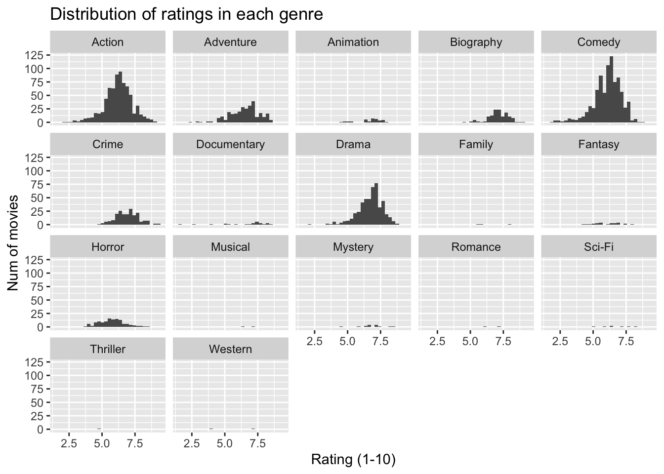
Using ggplot to find relationships between variables
Understanding the correlation between gross and cast_facebook_likes.
We have produced a scatterplot with Facebook Likes on the X-Axis and Gross Revenue on the Y-Axis.
ggplot(movies, aes(x = cast_facebook_likes, y = gross)) +
  geom_point() +
  geom_smooth(method = "lm")+
   labs(
    title = "Relationship of Facebook Likes vs Gross Revenue of the Movie",
    x = "Facebook Likes",
    y = "Gross Revenue"
  )+
  NULL
## `geom_smooth()` using formula 'y ~ x'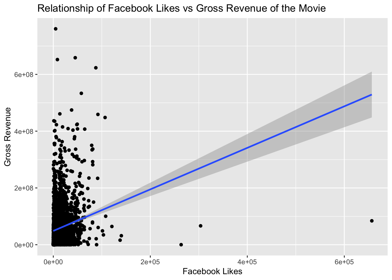 We analyze the following from the graph below-
- Facebook likes do not seem like a good indicator of the gross as there is no direct correlation as seen from the scatter plot.
- We mapped gross to Y axes and number of facebook likes to X, because the gross is the final outcome of a movie, aka dependent variable.
Now we examine the relationship between gross and budget by creating a scatterplot.
ggplot(movies, aes(x = budget , y = gross)) +
  geom_point() +
  geom_smooth(method = "lm") +
   labs(
    title = "Relationship of Gross Revenue vs Budget of the Movie",
    x = "Movie Budget",
    y = "Gross Revenue"
  )+
  NULL
## `geom_smooth()` using formula 'y ~ x'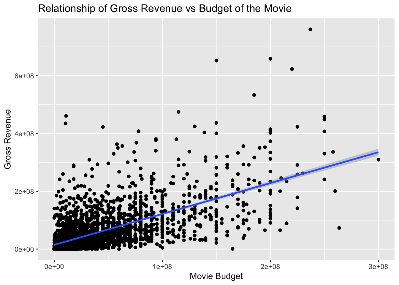
From the plot above we see that, the budget and gross do seem correlated. The higher the budget, it is more likely that the gross may be higher.
Furthermore, we examine the relationship between gross and rating.
Segmenting the scatterplot by ‘genre’, we can see the following results-
ggplot(movies, aes(x = rating , y = gross)) +
  geom_point() +
  geom_smooth(method = "lm") +
  facet_wrap(~genre) +
  labs(title = "Gross vs Rating of Movies For Each Genre ",
       x = "Rating",
       y = "Gross") +
  NULL
## `geom_smooth()` using formula 'y ~ x'## Warning in qt((1 - level)/2, df): NaNs produced
## Warning in qt((1 - level)/2, df): NaNs produced
## Warning in qt((1 - level)/2, df): NaNs produced## Warning in max(ids, na.rm = TRUE): no non-missing arguments to max; returning
## -Inf
## Warning in max(ids, na.rm = TRUE): no non-missing arguments to max; returning
## -Inf
## Warning in max(ids, na.rm = TRUE): no non-missing arguments to max; returning
## -Inf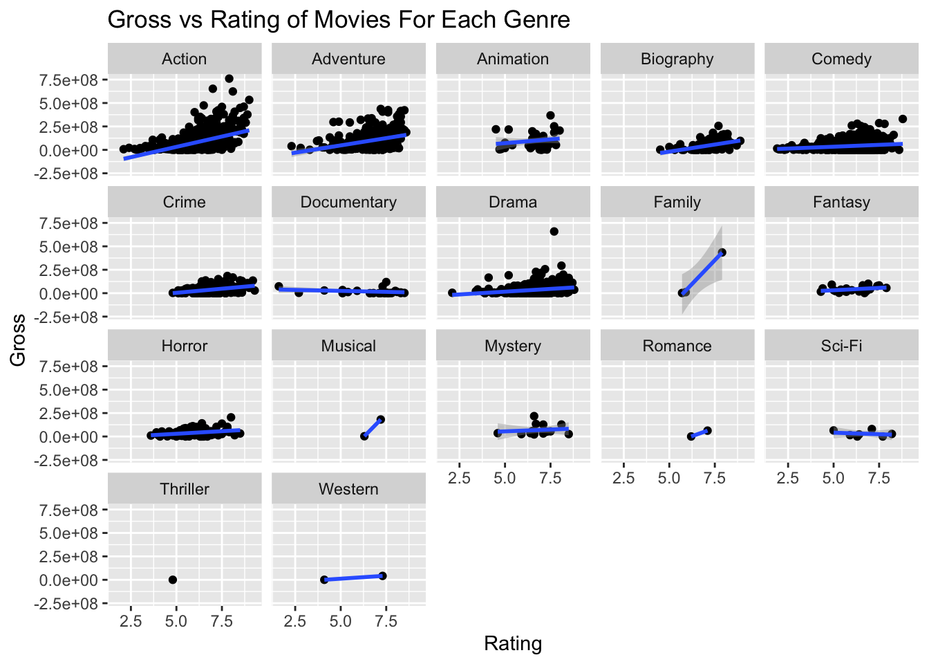
We can see that:
The higher the rating the more will be the gross for the most genres of movies.
For movies of some genres like ‘Documentary’, ‘Mystery’, ‘Horror’ and ‘Sci-Fi’, the gross has a very less change with respect to rating. Documentaries certainly have a different business model.
Negative correlation even appears.
Sample size of genres like ‘Family’, ‘Romance’ , ‘Musical’ is very small with under three values.