Youth Risk
Publish date: Sep 13, 2021Tags: R Data Analytics Data Visualization
Youth Risk Behavior Surveillance
Every two years, the Centers for Disease Control and Prevention conduct the Youth Risk Behavior Surveillance System (YRBSS) survey, where it takes data from high schoolers (9th through 12th grade), to analyze health patterns. We will work with a selected group of variables from a random sample of observations during one of the years the YRBSS was conducted.
Load the data
This data is part of the openintro textbook and we can load and inspect it. There are observations on 13 different variables, some categorical and some numerical. The meaning of each variable can be found by bringing up the help file:
?yrbssdata(yrbss)
glimpse(yrbss)## Rows: 13,583
## Columns: 13
## $ age <int> 14, 14, 15, 15, 15, 15, 15, 14, 15, 15, 15, 1…
## $ gender <chr> "female", "female", "female", "female", "fema…
## $ grade <chr> "9", "9", "9", "9", "9", "9", "9", "9", "9", …
## $ hispanic <chr> "not", "not", "hispanic", "not", "not", "not"…
## $ race <chr> "Black or African American", "Black or Africa…
## $ height <dbl> NA, NA, 1.73, 1.60, 1.50, 1.57, 1.65, 1.88, 1…
## $ weight <dbl> NA, NA, 84.37, 55.79, 46.72, 67.13, 131.54, 7…
## $ helmet_12m <chr> "never", "never", "never", "never", "did not …
## $ text_while_driving_30d <chr> "0", NA, "30", "0", "did not drive", "did not…
## $ physically_active_7d <int> 4, 2, 7, 0, 2, 1, 4, 4, 5, 0, 0, 0, 4, 7, 7, …
## $ hours_tv_per_school_day <chr> "5+", "5+", "5+", "2", "3", "5+", "5+", "5+",…
## $ strength_training_7d <int> 0, 0, 0, 0, 1, 0, 2, 0, 3, 0, 3, 0, 0, 7, 7, …
## $ school_night_hours_sleep <chr> "8", "6", "<5", "6", "9", "8", "9", "6", "<5"…Now we summarize the statistics of numerical variables, and create a very rough histogram.
skim(yrbss)| Name | yrbss |
| Number of rows | 13583 |
| Number of columns | 13 |
| _______________________ | |
| Column type frequency: | |
| character | 8 |
| numeric | 5 |
| ________________________ | |
| Group variables | None |
Variable type: character
| skim_variable | n_missing | complete_rate | min | max | empty | n_unique | whitespace |
|---|---|---|---|---|---|---|---|
| gender | 12 | 1.00 | 4 | 6 | 0 | 2 | 0 |
| grade | 79 | 0.99 | 1 | 5 | 0 | 5 | 0 |
| hispanic | 231 | 0.98 | 3 | 8 | 0 | 2 | 0 |
| race | 2805 | 0.79 | 5 | 41 | 0 | 5 | 0 |
| helmet_12m | 311 | 0.98 | 5 | 12 | 0 | 6 | 0 |
| text_while_driving_30d | 918 | 0.93 | 1 | 13 | 0 | 8 | 0 |
| hours_tv_per_school_day | 338 | 0.98 | 1 | 12 | 0 | 7 | 0 |
| school_night_hours_sleep | 1248 | 0.91 | 1 | 3 | 0 | 7 | 0 |
Variable type: numeric
| skim_variable | n_missing | complete_rate | mean | sd | p0 | p25 | p50 | p75 | p100 | hist |
|---|---|---|---|---|---|---|---|---|---|---|
| age | 77 | 0.99 | 16.16 | 1.26 | 12.00 | 15.00 | 16.00 | 17.00 | 18.00 | ▁▂▅▅▇ |
| height | 1004 | 0.93 | 1.69 | 0.10 | 1.27 | 1.60 | 1.68 | 1.78 | 2.11 | ▁▅▇▃▁ |
| weight | 1004 | 0.93 | 67.91 | 16.90 | 29.94 | 56.25 | 64.41 | 76.20 | 180.99 | ▆▇▂▁▁ |
| physically_active_7d | 273 | 0.98 | 3.90 | 2.56 | 0.00 | 2.00 | 4.00 | 7.00 | 7.00 | ▆▂▅▃▇ |
| strength_training_7d | 1176 | 0.91 | 2.95 | 2.58 | 0.00 | 0.00 | 3.00 | 5.00 | 7.00 | ▇▂▅▂▅ |
Exploratory Data Analysis
We first start with analyzing the weight of participants in kilograms. From the histogram and summary statistics below we can see the distribution of weights is positively skewed. We can see that the distribution is right skewed and there are 1004 missing values.
# stats
summary(yrbss$weight)
## Min. 1st Qu. Median Mean 3rd Qu. Max. NA's
## 29.94 56.25 64.41 67.91 76.20 180.99 1004# plot histogram
yrbss %>%
filter(!is.na(weight)) %>%
ggplot(aes(x=weight))+
geom_histogram(bins=30)+
NULL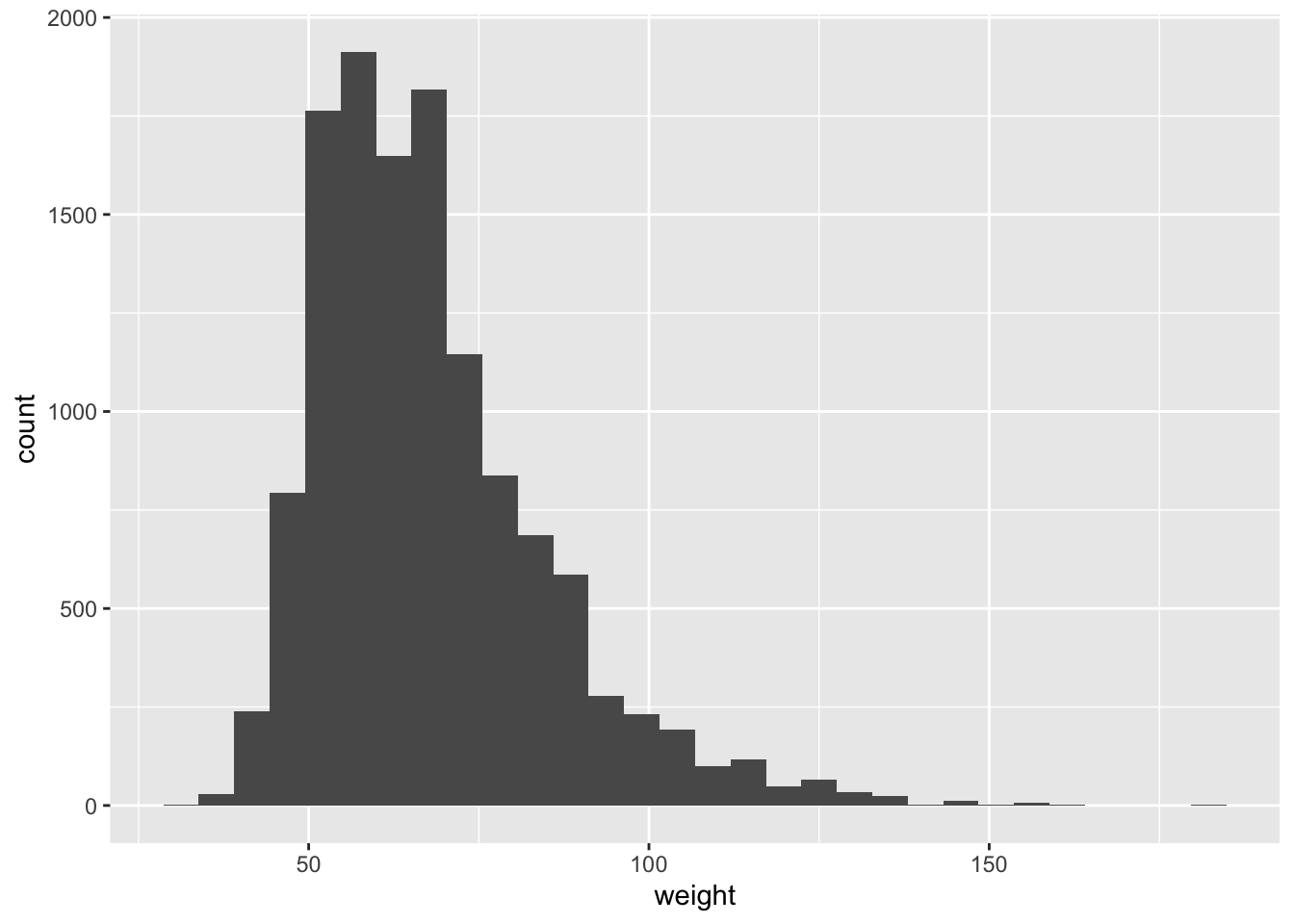
Next, consider the possible relationship between a high schooler’s weight and their physical activity. Next we plot the data to quickly visualize trends, identify strong associations, and develop research questions.
We create a new variable in the dataframe yrbss, called physical_3plus , which will be yes if they are physically active for at least 3 days a week, and no otherwise.
yrbss <- yrbss %>%
  mutate(physical_3plus = case_when(
    physically_active_7d >= 3 ~ "yes",
    physically_active_7d < 3 ~ "no",
    T ~ "NA"
  )) %>%
  filter(physical_3plus!="NA") # remove null values


# group by and summarise
yrbss_prop <- yrbss %>%
  group_by(physical_3plus) %>%
  summarise(n = n()) %>%
  mutate(prop= n/sum(n))

# another way: count
# yrbss_prop <- yrbss %>%
#  count(physical_3plus, sort=TRUE) %>%
#  mutate(prop= n/sum(n))
yrbss_prop
## # A tibble: 2 × 3
## physical_3plus n prop
## <chr> <int> <dbl>
## 1 no 4404 0.331
## 2 yes 8906 0.669Calculating confidence interval
# notes: here std_error is the standard deviation of the sample mean

not_prop <- yrbss_prop %>%
  filter(physical_3plus=="no") %>%
  pull("prop")

not_n <- yrbss_prop %>%
  filter(physical_3plus=="no") %>%
  pull("n")

# estimation of sd
std_error <- sqrt(not_prop * (1-not_prop) / (sum(yrbss_prop$n) ))

# with unknown population sd, use t distribution 1.960503
t_critical <- qt(0.975, not_n - 1)

margin_of_error <- t_critical * std_error

# ci
phy_3plus_low <- not_prop - margin_of_error
phy_3plus_high <- not_prop + margin_of_error

print(sprintf("95%% confidence interval is [%f,%f]",phy_3plus_low,phy_3plus_high))
## [1] "95% confidence interval is [0.322883,0.338875]"- 95% confidence interval for the population proportion of high schools that are NOT active 3 or more days per week is [0.322883,0.338875]
Boxplot
Next we make a boxplot of physical_3plus vs. weight to check the relationship between these two variables.
yrbss %>%
  filter(physical_3plus!="NA") %>%
  ggplot(aes(x = physical_3plus , y = weight)) +
  geom_boxplot()+
  labs(title = "Boxplot of Active for at least 3 days vs Weight",
       x = "Active at least 3 days",
       y = "Weight")+
  NULL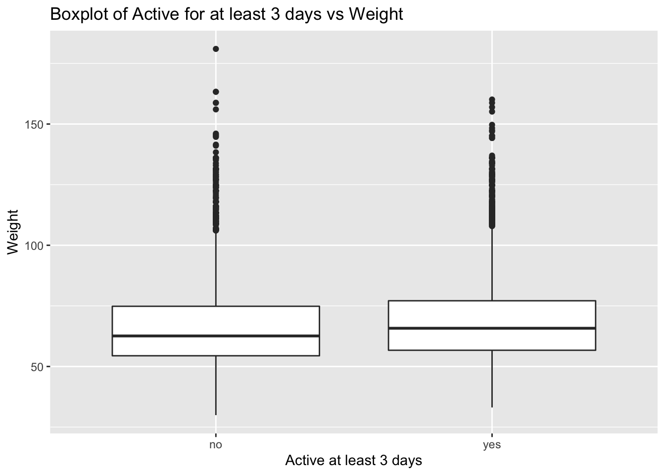
Conclusion: - No significant relationship can be identified. We expected the more students exercise the lighter weight they have. - But we can see that the median weight of the sample who are physically active for at least three days is greater than the median of the sample who are active for lesser than three days. This may be because of higher weight of muscle or bone due to working out/exercising.
Confidence Interval (Difference of means)
Boxplots show how the medians of the two distributions compare, but we can also compare the means of the distributions using either a confidence interval or a hypothesis test.
yrbss_stats <- favstats(weight~physical_3plus, data=yrbss,na.rm = T)

# use formulas
yrbss_stats_alt <- yrbss %>%
  group_by(physical_3plus) %>%
  summarise(avg_weight = mean(weight,na.rm=T),
            sd_weight_mean = sd(weight,na.rm=T),
            n=n())

#approximate by 1.96
t_critical <- 1.96 # qt(0.975, ) # calculate df with Welch-Satterhwaite formula

no_ci_lower <- 66.674 - t_critical*17.638/sqrt(sum(yrbss_stats_alt$n))
no_ci_higher <- 66.674 + t_critical*17.638/sqrt(sum(yrbss_stats_alt$n))
print(sprintf("weights of 'no': 95%% confidence interval is [%f,%f]",no_ci_lower,no_ci_higher))
## [1] "weights of 'no': 95% confidence interval is [66.374349,66.973651]"yes_ci_lower <- 68.448 - t_critical*16.478/sqrt(sum(yrbss_stats_alt$n))
yes_ci_higher <- 68.448 + t_critical*16.478/sqrt(sum(yrbss_stats_alt$n))
print(sprintf("weights of 'yes': 95%% confidence interval is [%f,%f]",yes_ci_lower,yes_ci_higher))## [1] "weights of 'yes': 95% confidence interval is [68.168056,68.727944]"- There is an observed difference of about 1.77kg (68.44 - 66.67), and we notice that the two confidence intervals do not overlap. It seems that the difference is at least 95% statistically significant. Let us also conduct a hypothesis test.
Hypothesis test with formula (Difference of means)
Null hypothesis \(H_0:\bar{weight}_{>=3h}-\bar{weight}_{<3h}=0\)
Alternative hypothesis \(H_1:\bar{weight}_{>=3h}-\bar{weight}_{<3h}\neq0\)
t.test(weight ~ physical_3plus, data = yrbss) # assume different variance##
## Welch Two Sample t-test
##
## data: weight by physical_3plus
## t = -5.353, df = 7478.8, p-value = 8.908e-08
## alternative hypothesis: true difference in means between group no and group yes is not equal to 0
## 95 percent confidence interval:
## -2.424441 -1.124728
## sample estimates:
## mean in group no mean in group yes
## 66.67389 68.44847Hypothesis test with infer
Next, we use hypothesize for conducting hypothesis tests.
First, we need to initialize the test, which we will save as obs_diff.
obs_diff <- yrbss %>%
  specify(weight ~ physical_3plus) %>%
  calculate(stat = "diff in means", order = c("yes", "no"))
## Warning: Removed 946 rows containing missing values.obs_diff## Response: weight (numeric)
## Explanatory: physical_3plus (factor)
## # A tibble: 1 × 1
## stat
## <dbl>
## 1 1.77The statistic we are searching for is the difference in means, with the order being yes - no != 0.
After initializing the test, we will simulate the test on the null distribution, which we will save as null.
null_dist <- yrbss %>%
  # specify variables
  specify(weight ~ physical_3plus) %>%

  # assume independence, i.e, there is no difference
  hypothesize(null = "independence") %>%

  # generate 1000 reps, of type "permute"
  generate(reps = 1000, type = "permute") %>%

  # calculate statistic of difference, namely "diff in means"
  calculate(stat = "diff in means", order = c("yes", "no"))
## Warning: Removed 946 rows containing missing values.We can visualize this null distribution with the following code:
ggplot(data = null_dist, aes(x = stat)) +
  geom_histogram()+
  NULL
## `stat_bin()` using `bins = 30`. Pick better value with `binwidth`.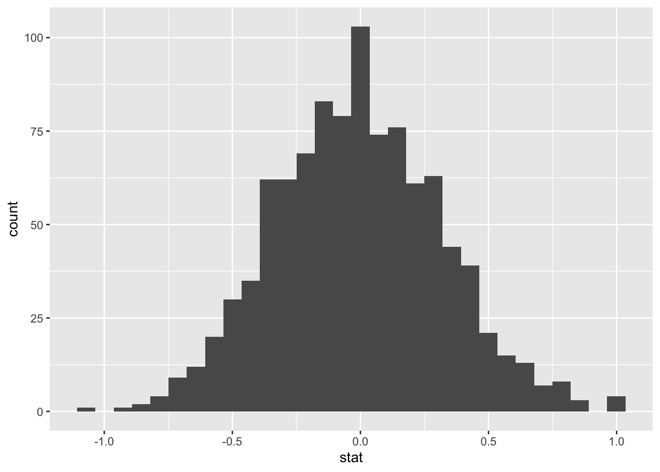
Now that the test is initialized and the null distribution formed, we will visualise to see how many of these null permutations have a difference of at least obs_stat of 1.77. We will also calculate the p-value for the hypothesis test using the function infer::get_p_value().
null_dist %>% visualize() +
  shade_p_value(obs_stat = obs_diff, direction = "two-sided")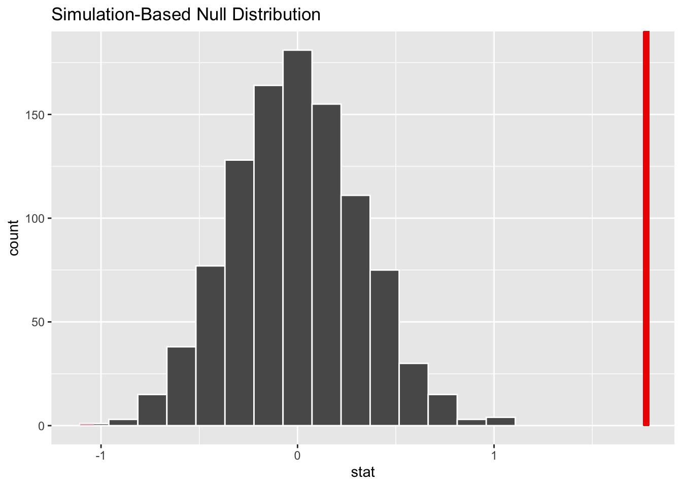
null_dist %>%
  get_p_value(obs_stat = obs_diff, direction = "two_sided")
## Warning: Please be cautious in reporting a p-value of 0. This result is an
## approximation based on the number of `reps` chosen in the `generate()` step. See
## `?get_p_value()` for more information.## # A tibble: 1 × 1
## p_value
## <dbl>
## 1 0Findings:
- In 1000 permutations, there is no point has a difference of at least obs_stat of 1.77. The p-value here is given by 0, but this result is an approximation based on the number of reps chosen in the generate() step.
- Since the p_value is close to 0, we will reject the null hypothesis.