Data Science I, Workshop I: Predicting interest rates at the Lending Club
Publish date: Oct 12, 2021Table of contents
- Q1 Exploratory data analysis and visualisation
- Q2 Analysis on model 1 (questions about model 1)
- Q3 Analysis on model 2-5 (questions about model 2-5)
- Q4 Predictive accuracy of Model 2
- Q5 Comparison between 10-fold cross validation and hold-out method
- Q6 Analysis on learning curves
- Q7 Comparison between OLS regression and LASSO
- Q8 Prediction improvement by adding time information
- Q9 Explanatory power of bond yields
- Q10 Model Comparison
- Q11 Further improvements
- Analysis on additional data
Load and prepare the data
We start by loading the data to R in a dataframe.
lc_raw <- read_csv(here::here("data","LendingClub Data.csv"),  skip=1) %>%  #since the first row is a title we want to skip it.
  clean_names() # use janitor::clean_names()
ICE the data: Inspect, Clean, Explore
lc_clean<- lc_raw %>%
  dplyr::select(-x20:-x80) %>% #delete empty columns
  filter(!is.na(int_rate)) %>%   #delete empty rows
  mutate(
    issue_d = mdy(issue_d),  # lubridate::mdy() to fix date format
    term = factor(term_months),     # turn 'term' into a categorical variable
    delinq_2yrs = factor(delinq_2yrs) # turn 'delinq_2yrs' into a categorical variable
  ) %>%
  dplyr::select(-emp_title,-installment, -term_months, everything()) #move some not-so-important variables to the end.
The data is now in a clean format stored in the dataframe “lc_clean.”
Q1 Exploratory data analysis and visualisation
# Build a histogram of interest rates.
ggplot(lc_clean, aes(x=int_rate))+
  geom_histogram(binwidth=0.01)+
  scale_x_continuous(labels = scales::percent) +
  labs(x="Interest Rate", title = "Distribution of Interest Rates")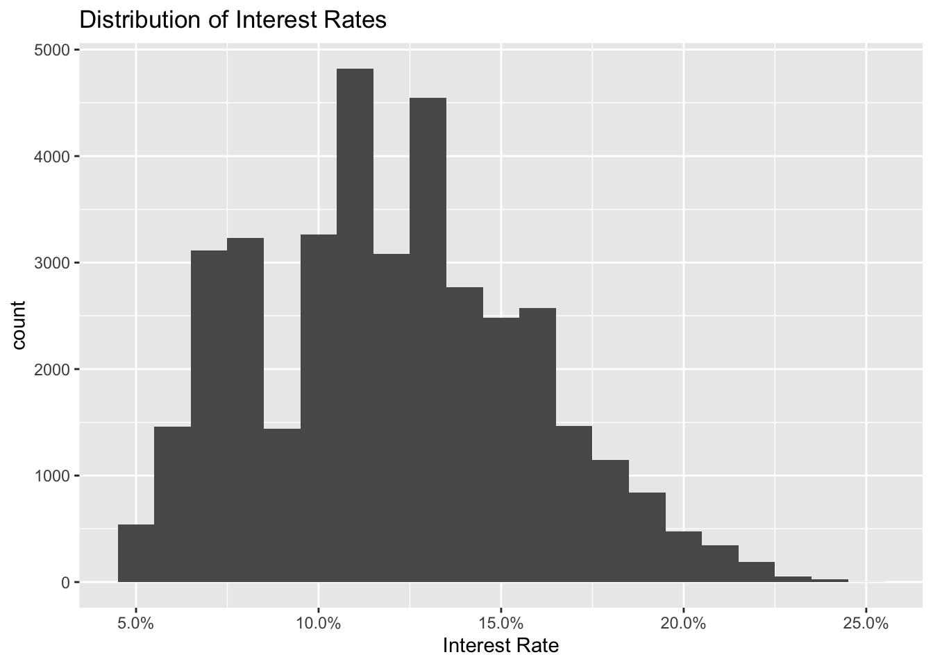
# Build a histogram of interest rates but use different color for loans of different grades
ggplot(lc_clean, aes(x=int_rate, fill=grade))+
  geom_histogram(binwidth=0.01)+scale_x_continuous(labels = scales::percent)+
labs(x="Interest Rate", title = "Distribution of Interest Rates by Grade") 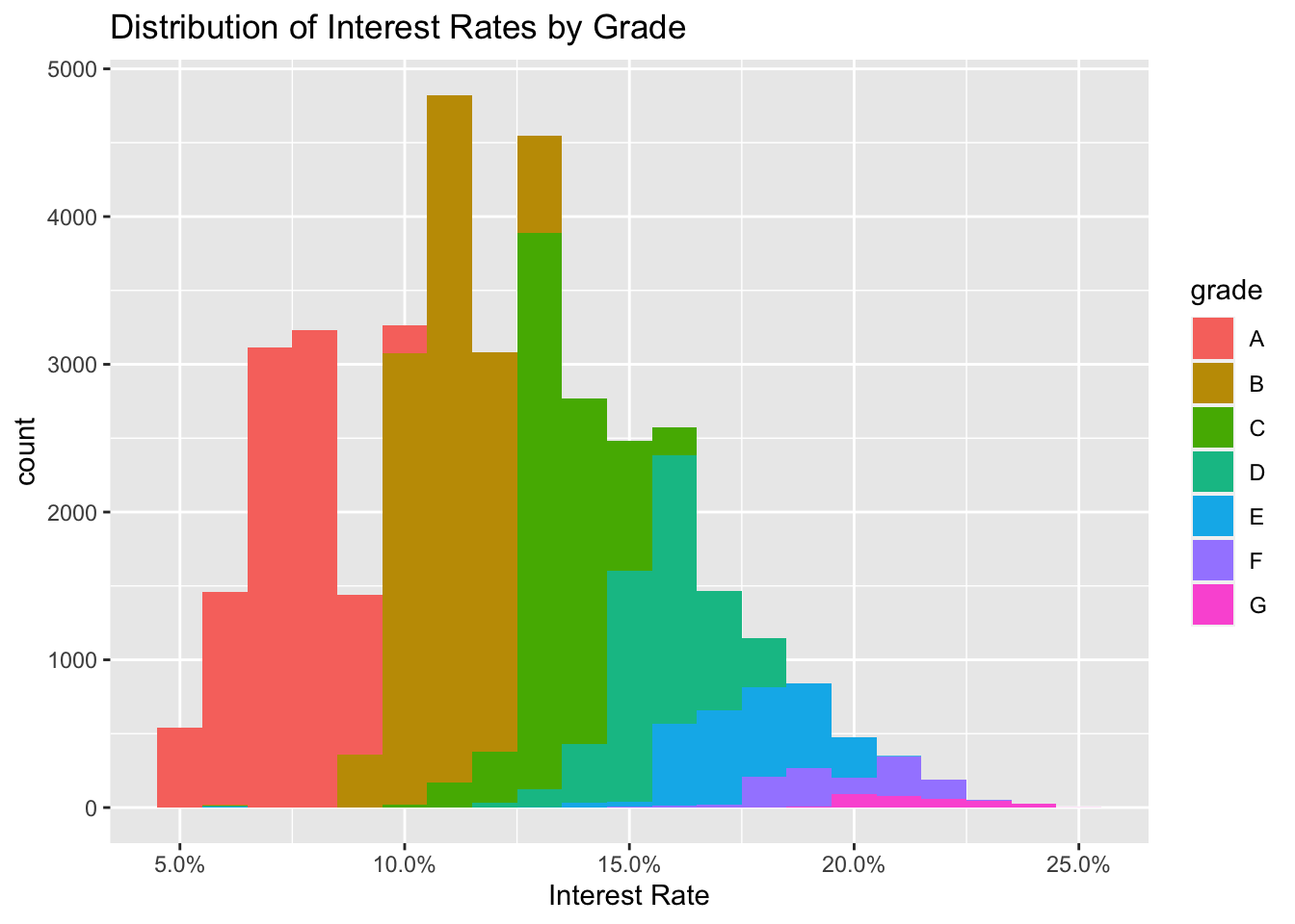
# Produce a scatter plot of loan amount against interest rate and add visually the line of best fit
ggplot(lc_clean[seq(1, nrow(lc_clean), 10), ] , aes(y=int_rate, x=loan_amnt)) +
  geom_point(size=0.1, alpha=0.5)+
  geom_smooth(method="lm", se=0) +
  labs(y="Interest Rate", x="Loan Amount ($)", title = "Comparing Interest Rates and Loan Amounts")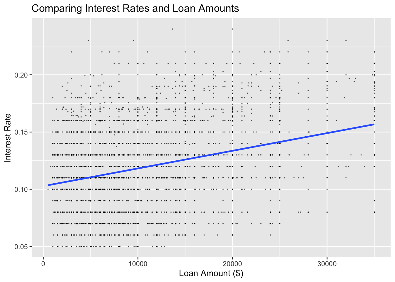
# Produce a scatter plot of annual income against interest rate and add visually the line of best fit
ggplot(lc_clean[seq(1, nrow(lc_clean), 10), ] , aes(y=int_rate, x=annual_inc)) +
  geom_point(size=0.1)+
  geom_smooth(method="lm", se=0) +
  labs(y="Interest Rate", x="Annual Income ($)", title="Comparing Interest Rates and Annual Income")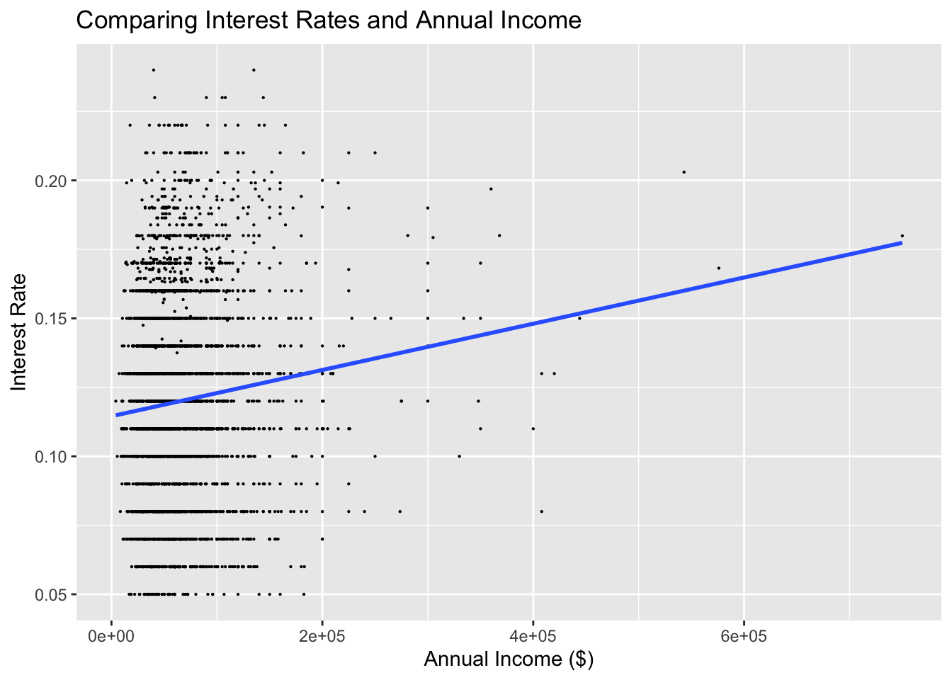
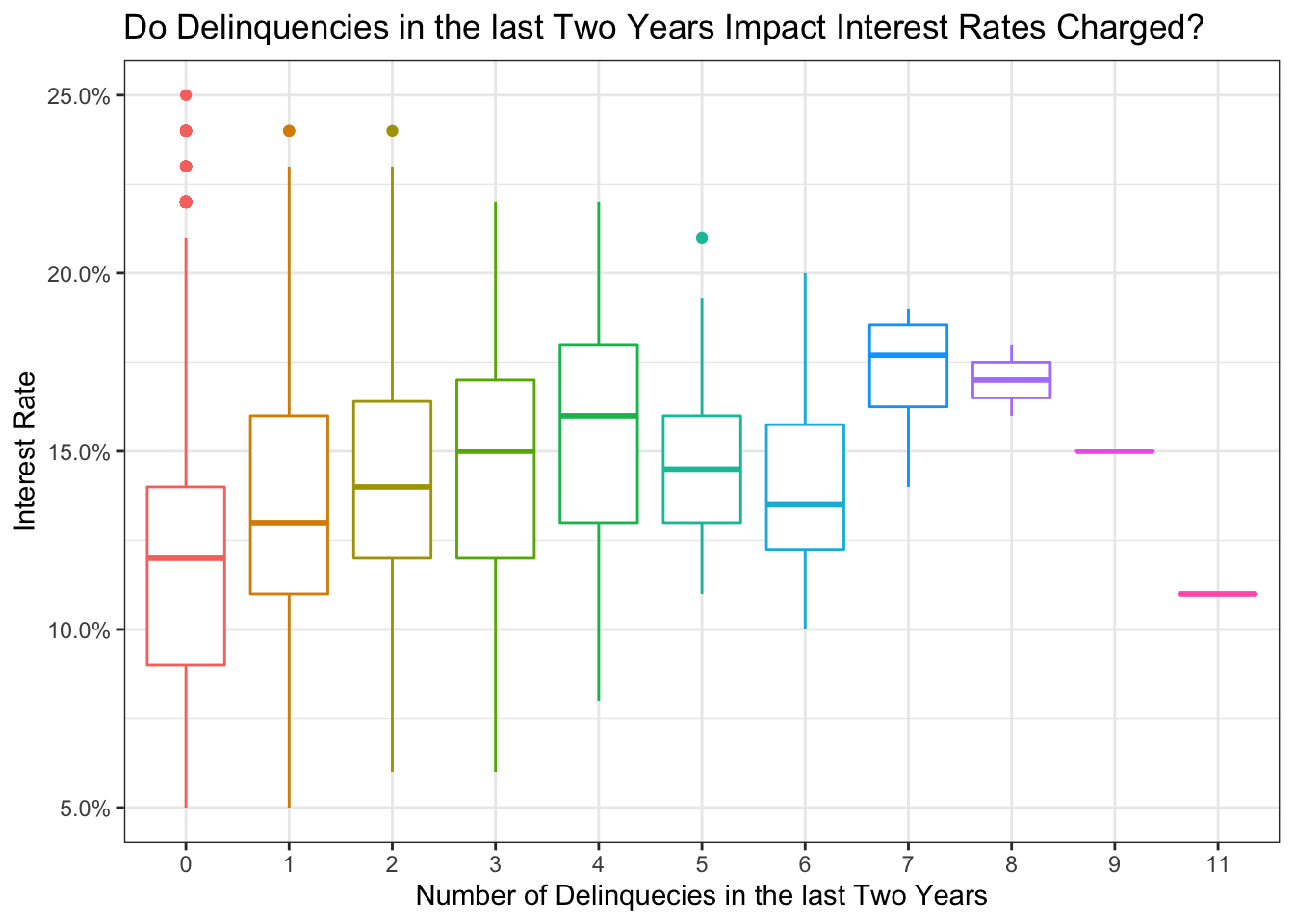
# In the same axes, produce box plots of the interest rate for every value of delinquencies
ggplot(lc_clean , aes(y=int_rate, x=delinq_2yrs, colour= delinq_2yrs)) +
  geom_boxplot()+
  # geom_jitter()+
  theme_bw()+
   scale_y_continuous(labels=scales::percent)+
  theme(legend.position = "none")+
  labs(
    title = "Do Delinquencies in the last Two Years Impact Interest Rates Charged?",
    x= "Number of Delinquecies in the last Two Years", y="Interest Rate"
  )
ggplot(lc_clean, aes (y=int_rate, x=issue_d, color = grade))+
  geom_point()+
  theme_bw()+
  labs(title="Interest Rate Evolution Over Time by Grade", x="Issue Date", y="Interest Rate")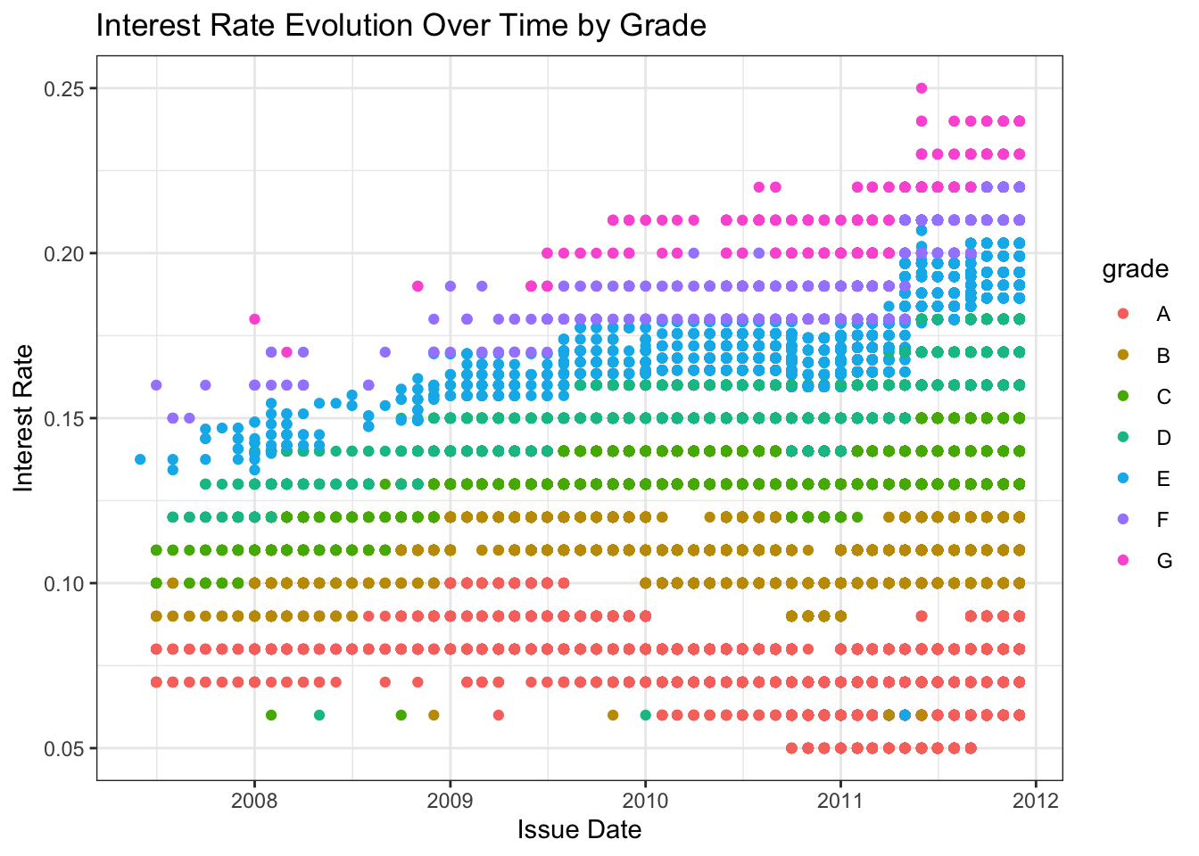
lc_clean %>%
  group_by (home_ownership) %>%
  summarize (mean_int = mean(int_rate)) %>%
  ggplot (aes(x = home_ownership, y= mean_int))+geom_col()+
  labs (title = "Relationship between Home Ownership and Interest Rates", x="Home Ownership Status", y="Interest Rate")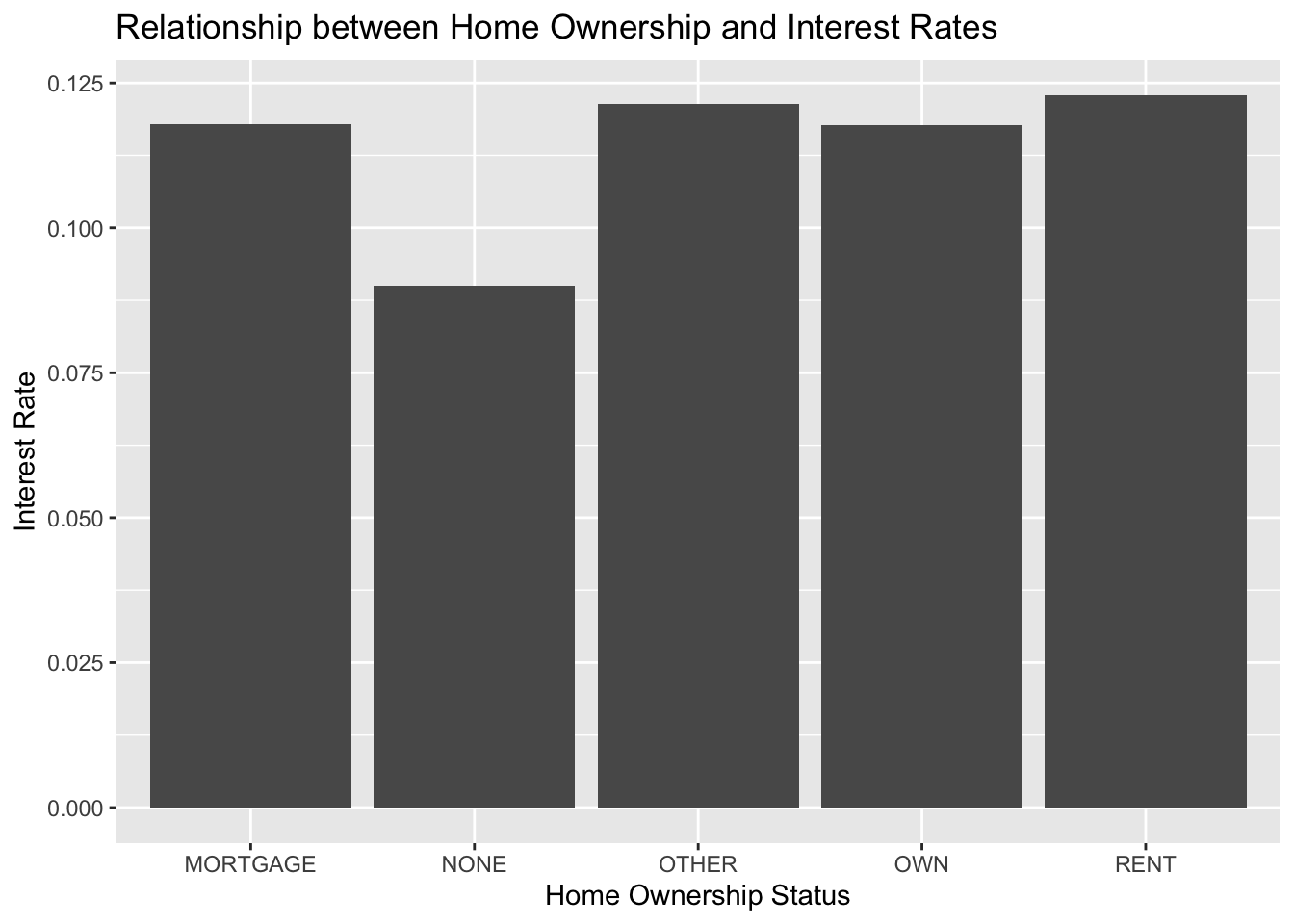
Estimate simple linear regression models
We start with a simple but quite powerful model.
# Use the lm command to estimate a regression model with the following variables "loan_amnt",  "term", "dti", "annual_inc", and "grade"

model1<-lm(int_rate ~ loan_amnt + term + dti + annual_inc + grade, data = lc_clean
  )
summary(model1)
##
## Call:
## lm(formula = int_rate ~ loan_amnt + term + dti + annual_inc +
## grade, data = lc_clean)
##
## Residuals:
## Min 1Q Median 3Q Max
## -0.118827 -0.007035 -0.000342 0.006828 0.035081
##
## Coefficients:
## Estimate Std. Error t value Pr(>|t|)
## (Intercept) 7.169e-02 1.689e-04 424.363 < 2e-16 ***
## loan_amnt 1.475e-07 8.284e-09 17.809 < 2e-16 ***
## term60 3.608e-03 1.419e-04 25.431 < 2e-16 ***
## dti 4.328e-05 8.269e-06 5.234 1.66e-07 ***
## annual_inc -9.734e-10 9.283e-10 -1.049 0.294
## gradeB 3.554e-02 1.492e-04 238.248 < 2e-16 ***
## gradeC 6.016e-02 1.658e-04 362.783 < 2e-16 ***
## gradeD 8.172e-02 1.906e-04 428.746 < 2e-16 ***
## gradeE 9.999e-02 2.483e-04 402.660 < 2e-16 ***
## gradeF 1.195e-01 3.673e-04 325.408 < 2e-16 ***
## gradeG 1.355e-01 6.208e-04 218.245 < 2e-16 ***
## ---
## Signif. codes: 0 '***' 0.001 '**' 0.01 '*' 0.05 '.' 0.1 ' ' 1
##
## Residual standard error: 0.01056 on 37858 degrees of freedom
## Multiple R-squared: 0.9198, Adjusted R-squared: 0.9197
## F-statistic: 4.34e+04 on 10 and 37858 DF, p-value: < 2.2e-16Q2 Analysis on model 1 (questions about model 1)
- Are all variables statistically significant?
- All the values are statistically significant except for annual income. The P values for all variables are less than 0.05, but the P value for annual income is larder than 0.05.
- Interpret all the coefficients in the regression.
- For all the coefficients in this equation, its interpretation is that if the loan amount increases by 100,000 the interest rate will increase by 1.5%.
- Additionally, if the loan term is 60 months, the interest rate of the loan will be higher than that of a 36 month loan by on average 0.36%. Futhermore, a one unit increase to the debt-to-income ratio will increase on average the loan interest rate by 0.0043%.
- Annual income is insignificant. Finally, comparing to Grade A, lowering the grade by each additional letter mean that the on average the interest rate will increase by 3.55% for Grabe B, 6.02% for Grade C, 8.17% for Grade D, 10% for Grade E, 12% for Grade F, and 14% for Grade G.
- How much explanatory power does the model have?
- The model has an adjusted R squared of .9197. This means that the model can explain about 92% of the varibility of the interest rates with this data.
- How wide would the 95% confidence interval of any prediction based on this model be?
- The confidence interval width is 4%, which is a high number when trying to predit interest rates.
Feature Engineering
Then we built progressively more complex models, with more features.
#Add to model 1 an interaction between loan amount and grade. Use the "var1*var2" notation to define an interaction term in the linear regression model. This will add the interaction and the individual variables to the model.

model2 <- lm(int_rate ~ loan_amnt*grade + term +dti + annual_inc, data = lc_clean)
summary(model2)
##
## Call:
## lm(formula = int_rate ~ loan_amnt * grade + term + dti + annual_inc,
## data = lc_clean)
##
## Residuals:
## Min 1Q Median 3Q Max
## -0.119807 -0.007230 -0.000057 0.006588 0.037460
##
## Coefficients:
## Estimate Std. Error t value Pr(>|t|)
## (Intercept) 7.171e-02 2.345e-04 305.762 < 2e-16 ***
## loan_amnt 1.528e-07 2.028e-08 7.537 4.91e-14 ***
## gradeB 3.623e-02 2.732e-04 132.619 < 2e-16 ***
## gradeC 6.198e-02 2.988e-04 207.452 < 2e-16 ***
## gradeD 8.082e-02 3.483e-04 232.034 < 2e-16 ***
## gradeE 9.633e-02 4.625e-04 208.293 < 2e-16 ***
## gradeF 1.143e-01 7.735e-04 147.699 < 2e-16 ***
## gradeG 1.327e-01 1.551e-03 85.580 < 2e-16 ***
## term60 3.793e-03 1.424e-04 26.636 < 2e-16 ***
## dti 3.836e-05 8.250e-06 4.649 3.34e-06 ***
## annual_inc -1.224e-09 9.249e-10 -1.324 0.18564
## loan_amnt:gradeB -6.617e-08 2.441e-08 -2.710 0.00673 **
## loan_amnt:gradeC -1.704e-07 2.621e-08 -6.500 8.14e-11 ***
## loan_amnt:gradeD 6.703e-08 2.798e-08 2.395 0.01662 *
## loan_amnt:gradeE 2.209e-07 3.016e-08 7.323 2.47e-13 ***
## loan_amnt:gradeF 2.779e-07 4.136e-08 6.720 1.85e-11 ***
## loan_amnt:gradeG 1.265e-07 7.260e-08 1.743 0.08140 .
## ---
## Signif. codes: 0 '***' 0.001 '**' 0.01 '*' 0.05 '.' 0.1 ' ' 1
##
## Residual standard error: 0.01052 on 37852 degrees of freedom
## Multiple R-squared: 0.9204, Adjusted R-squared: 0.9204
## F-statistic: 2.735e+04 on 16 and 37852 DF, p-value: < 2.2e-16#Add to the model we just created above the square and the cube of annual income. Use the poly(var_name,3) command as a variable in the linear regression model.
model3 <- lm(int_rate ~ loan_amnt*grade + term +dti + poly(annual_inc,3), data = lc_clean)
summary(model3)##
## Call:
## lm(formula = int_rate ~ loan_amnt * grade + term + dti + poly(annual_inc,
## 3), data = lc_clean)
##
## Residuals:
## Min 1Q Median 3Q Max
## -0.119814 -0.007238 -0.000065 0.006594 0.037471
##
## Coefficients:
## Estimate Std. Error t value Pr(>|t|)
## (Intercept) 7.161e-02 2.279e-04 314.200 < 2e-16 ***
## loan_amnt 1.556e-07 2.047e-08 7.600 3.03e-14 ***
## gradeB 3.623e-02 2.732e-04 132.611 < 2e-16 ***
## gradeC 6.198e-02 2.988e-04 207.398 < 2e-16 ***
## gradeD 8.081e-02 3.483e-04 231.999 < 2e-16 ***
## gradeE 9.633e-02 4.625e-04 208.283 < 2e-16 ***
## gradeF 1.143e-01 7.736e-04 147.695 < 2e-16 ***
## gradeG 1.327e-01 1.551e-03 85.573 < 2e-16 ***
## term60 3.786e-03 1.426e-04 26.546 < 2e-16 ***
## dti 3.761e-05 8.294e-06 4.535 5.79e-06 ***
## poly(annual_inc, 3)1 -1.589e-02 1.117e-02 -1.423 0.1549
## poly(annual_inc, 3)2 6.296e-03 1.086e-02 0.580 0.5621
## poly(annual_inc, 3)3 -8.981e-03 1.084e-02 -0.828 0.4076
## loan_amnt:gradeB -6.633e-08 2.442e-08 -2.717 0.0066 **
## loan_amnt:gradeC -1.703e-07 2.621e-08 -6.498 8.23e-11 ***
## loan_amnt:gradeD 6.709e-08 2.798e-08 2.398 0.0165 *
## loan_amnt:gradeE 2.209e-07 3.016e-08 7.324 2.45e-13 ***
## loan_amnt:gradeF 2.780e-07 4.136e-08 6.722 1.82e-11 ***
## loan_amnt:gradeG 1.270e-07 7.260e-08 1.750 0.0801 .
## ---
## Signif. codes: 0 '***' 0.001 '**' 0.01 '*' 0.05 '.' 0.1 ' ' 1
##
## Residual standard error: 0.01052 on 37850 degrees of freedom
## Multiple R-squared: 0.9204, Adjusted R-squared: 0.9204
## F-statistic: 2.431e+04 on 18 and 37850 DF, p-value: < 2.2e-16#Continuing with the previous model, instead of annual income as a continuous variable break it down into quartiles and use quartile dummy variables.
lc_clean <- lc_clean %>%
mutate(quartiles_annual_inc = as.factor(ntile(annual_inc, 4)))
model4 <-lm(int_rate ~ loan_amnt*grade + term +dti + quartiles_annual_inc, data = lc_clean)
summary(model4) ##
## Call:
## lm(formula = int_rate ~ loan_amnt * grade + term + dti + quartiles_annual_inc,
## data = lc_clean)
##
## Residuals:
## Min 1Q Median 3Q Max
## -0.119767 -0.007203 -0.000064 0.006596 0.037581
##
## Coefficients:
## Estimate Std. Error t value Pr(>|t|)
## (Intercept) 7.187e-02 2.414e-04 297.700 < 2e-16 ***
## loan_amnt 1.615e-07 2.048e-08 7.889 3.13e-15 ***
## gradeB 3.622e-02 2.733e-04 132.524 < 2e-16 ***
## gradeC 6.196e-02 2.989e-04 207.272 < 2e-16 ***
## gradeD 8.079e-02 3.484e-04 231.877 < 2e-16 ***
## gradeE 9.632e-02 4.625e-04 208.273 < 2e-16 ***
## gradeF 1.143e-01 7.735e-04 147.723 < 2e-16 ***
## gradeG 1.327e-01 1.551e-03 85.570 < 2e-16 ***
## term60 3.781e-03 1.425e-04 26.532 < 2e-16 ***
## dti 3.672e-05 8.259e-06 4.446 8.78e-06 ***
## quartiles_annual_inc2 -2.619e-04 1.548e-04 -1.692 0.09068 .
## quartiles_annual_inc3 -3.992e-04 1.590e-04 -2.510 0.01208 *
## quartiles_annual_inc4 -5.382e-04 1.692e-04 -3.181 0.00147 **
## loan_amnt:gradeB -6.638e-08 2.441e-08 -2.719 0.00655 **
## loan_amnt:gradeC -1.699e-07 2.621e-08 -6.483 9.10e-11 ***
## loan_amnt:gradeD 6.770e-08 2.798e-08 2.419 0.01555 *
## loan_amnt:gradeE 2.203e-07 3.016e-08 7.304 2.85e-13 ***
## loan_amnt:gradeF 2.766e-07 4.136e-08 6.687 2.30e-11 ***
## loan_amnt:gradeG 1.267e-07 7.259e-08 1.746 0.08089 .
## ---
## Signif. codes: 0 '***' 0.001 '**' 0.01 '*' 0.05 '.' 0.1 ' ' 1
##
## Residual standard error: 0.01052 on 37850 degrees of freedom
## Multiple R-squared: 0.9204, Adjusted R-squared: 0.9204
## F-statistic: 2.432e+04 on 18 and 37850 DF, p-value: < 2.2e-16#Compare the performance of these four models using the anova command
anova(model1, model2, model3, model4)| Res.Df | RSS | Df | Sum of Sq | F | Pr(>F) |
|---|---|---|---|---|---|
| 3.79e+04 | 4.22 | ||||
| 3.79e+04 | 4.19 | 6 | 0.0332 | 50 | 1.64e-61 |
| 3.78e+04 | 4.19 | 2 | 0.000107 | 0.484 | 0.616 |
| 3.78e+04 | 4.19 | 0 | 0.000915 |
Q3 Analysis on model 2-5 (questions about model 2-5)
- Which of the four models has the most explanatory power in sample?
- When looking at the anova output, you can see that the R squared is increasing from each additional model, ending with an R-Squared of 92.04% for model 4, which we believe to have the most explanatory power.
- Also, when looking at the variables, model 4 has the most number of significant variables, while model 1,2 and 3 have a higher number of insignificant variables. This is partly due to the fact that the quartiles for annual income are more significant than annual income alone and the polynomial of annual income.
- In model 2, how can we interpret the estimated coefficient of the interaction term between grade B and loan amount?
- The effect of increasing the loan amount is different for each grade. Using this interaction, we can see how the different Grades effect the interest rates taking into account the loan amount.
- The problem of multicollinearity describes situations in which one feature is correlated with other features (or with a linear combination of other features). If the goal is to use the model to make predictions, should we be concerned about multicollinearity? Why, or why not?
- When making predictions, multicollinearity is not an issue we need to worry about. All we care about is how good our prediction is, not how each variable effects the output.
Out of sample testing
We want to check the predictive accuracy of model2 by holding out a subset of the data to use as a testing data set. This method is sometimes referred to as the hold-out method for out-of-sample testing.
# split the data in dataframe called "testing" and another one called  "training". The "training" dataframe should have 80% of the data and the "testing" dataframe 20%.

set.seed(1235)

train_test_split <- initial_split(lc_clean, prop = 0.80) # split the dataset into training (80% of data points) and testing (20% of data points) datasets
testing <- testing(train_test_split)
training <- training(train_test_split)

# Fit model2 on the training set
model2_training<-lm(int_rate ~ loan_amnt + term+ dti + annual_inc + grade +grade:loan_amnt, training)

# Calculate the RMSE of the model in the training set (in sample)
rmse_training<-sqrt(mean((residuals(model2_training))^2))

print(rmse_training)
## [1] 0.01051954# Use the model to make predictions out of sample in the testing set
pred<-predict(model2_training,testing)
# Calculate the RMSE of the model in the testing set (out of sample)
rmse_testing<- RMSE(pred,testing$int_rate)
print(rmse_testing)## [1] 0.01049407print(rmse_training - rmse_testing) # comparing the training and testing result of RMSE## [1] 2.546534e-05Q4 Predictive accuracy of Model 2
- The predictive accuracy changes by .0001, which is basically zero. This is sensitive to the random seed chosen because RMSE changes when changeing the random seed. Finally, our RMSE is very similar in out training and testing set, giving us confidence that there is no evidence of overfitting.
k-fold cross validation
We can also do out of sample testing using the method of k-fold cross validation. Using the caret package this is easy.
#the method "cv" stands for cross validation. We re going to create 10 folds.

control <- trainControl (
    method="cv",
    number=10,
    verboseIter=TRUE) #by setting this to true the model will report its progress after each estimation

#we are going to train the model and report the results using k-fold cross validation

plsFit<-train(
    int_rate ~ loan_amnt + term+ dti + annual_inc + grade +grade:loan_amnt ,
    lc_clean,
   method = "lm",
    trControl = control
   )
## + Fold01: intercept=TRUE
## - Fold01: intercept=TRUE
## + Fold02: intercept=TRUE
## - Fold02: intercept=TRUE
## + Fold03: intercept=TRUE
## - Fold03: intercept=TRUE
## + Fold04: intercept=TRUE
## - Fold04: intercept=TRUE
## + Fold05: intercept=TRUE
## - Fold05: intercept=TRUE
## + Fold06: intercept=TRUE
## - Fold06: intercept=TRUE
## + Fold07: intercept=TRUE
## - Fold07: intercept=TRUE
## + Fold08: intercept=TRUE
## - Fold08: intercept=TRUE
## + Fold09: intercept=TRUE
## - Fold09: intercept=TRUE
## + Fold10: intercept=TRUE
## - Fold10: intercept=TRUE
## Aggregating results
## Fitting final model on full training setsummary(plsFit)##
## Call:
## lm(formula = .outcome ~ ., data = dat)
##
## Residuals:
## Min 1Q Median 3Q Max
## -0.119807 -0.007230 -0.000057 0.006588 0.037460
##
## Coefficients:
## Estimate Std. Error t value Pr(>|t|)
## (Intercept) 7.171e-02 2.345e-04 305.762 < 2e-16 ***
## loan_amnt 1.528e-07 2.028e-08 7.537 4.91e-14 ***
## term60 3.793e-03 1.424e-04 26.636 < 2e-16 ***
## dti 3.836e-05 8.250e-06 4.649 3.34e-06 ***
## annual_inc -1.224e-09 9.249e-10 -1.324 0.18564
## gradeB 3.623e-02 2.732e-04 132.619 < 2e-16 ***
## gradeC 6.198e-02 2.988e-04 207.452 < 2e-16 ***
## gradeD 8.082e-02 3.483e-04 232.034 < 2e-16 ***
## gradeE 9.633e-02 4.625e-04 208.293 < 2e-16 ***
## gradeF 1.143e-01 7.735e-04 147.699 < 2e-16 ***
## gradeG 1.327e-01 1.551e-03 85.580 < 2e-16 ***
## `loan_amnt:gradeB` -6.617e-08 2.441e-08 -2.710 0.00673 **
## `loan_amnt:gradeC` -1.704e-07 2.621e-08 -6.500 8.14e-11 ***
## `loan_amnt:gradeD` 6.703e-08 2.798e-08 2.395 0.01662 *
## `loan_amnt:gradeE` 2.209e-07 3.016e-08 7.323 2.47e-13 ***
## `loan_amnt:gradeF` 2.779e-07 4.136e-08 6.720 1.85e-11 ***
## `loan_amnt:gradeG` 1.265e-07 7.260e-08 1.743 0.08140 .
## ---
## Signif. codes: 0 '***' 0.001 '**' 0.01 '*' 0.05 '.' 0.1 ' ' 1
##
## Residual standard error: 0.01052 on 37852 degrees of freedom
## Multiple R-squared: 0.9204, Adjusted R-squared: 0.9204
## F-statistic: 2.735e+04 on 16 and 37852 DF, p-value: < 2.2e-16#the method "cv" stands for cross validation. We re going to create 10 folds.
control <- trainControl (
method="cv",
number=5,
verboseIter=TRUE) #by setting this to true the model will report its progress after each estimation
#we are going to train the model and report the results using k-fold cross validation
plsFit<-train(
int_rate ~ loan_amnt + term+ dti + annual_inc + grade +grade:loan_amnt ,
lc_clean,
method = "lm",
trControl = control
)
summary(plsFit)#the method "cv" stands for cross validation. We re going to create 10 folds.
control <- trainControl (
method="cv",
number=15,
verboseIter=TRUE) #by setting this to true the model will report its progress after each estimation
#we are going to train the model and report the results using k-fold cross validation
plsFit<-train(
int_rate ~ loan_amnt + term+ dti + annual_inc + grade +grade:loan_amnt ,
lc_clean,
method = "lm",
trControl = control
)
summary(plsFit)Q5 Comparison between 10-fold cross validation and hold-out method
The RMSE of the hold out method for our training set was 0.01052 while the RMSE for the 10-fold cross validation is 0.01
10-fold cross is more reliable of a method as it uses all the data set as training and testing. The hold-out method reduces the data we use for training as it sets aside some data for the testing method. So, if we have a small data set, the data set we hold out can wrongly represent the whole data set. This gives us the option of using all the data points. A drawback for 10-fold is the time it takes to run it K amount of times.
When running the 5-fold and 15-fold models, we get the same RMSE and R squared as the 10-fold. This means that the model is very robust.
Sample size estimation and learning curves
- We can use the hold out method for out-of-sample testing to check if we have a sufficiently large sample to estimate the model reliably.
- The idea is to set aside some of the data as a testing set. From the remaining data draw progressively larger training sets and check how the performance of the model on the testing set changes. If the performance no longer improves with larger training sets we know we have a large enough sample. The code below does this. Examine it and run it with different random seeds.
#select a testing dataset (25% of all data)
set.seed(12)

train_test_split <- initial_split(lc_clean, prop = 0.75)
remaining <- training(train_test_split)
testing <- testing(train_test_split)

#We are now going to run 30 models starting from a tiny training set drawn from the training data and progressively increasing its size. The testing set remains the same in all iterations.

#initiating the model by setting some parameters to zero
rmse_sample <- 0
sample_size<-0
Rsq_sample<-0

for(i in 1:30) {
#from the remaining dataset select a smaller subset to training the data
set.seed(100)
sample

  learning_split <- initial_split(remaining, prop = i/200)
  training <- training(learning_split)
  sample_size[i]=nrow(training)

  #traing the model on the small dataset
  model3<-lm(int_rate ~ loan_amnt + term+ dti + annual_inc + grade + grade:loan_amnt, training)
  #test the performance of the model on the large testing dataset. This stays fixed for all iterations.
  pred<-predict(model3,testing)
  rmse_sample[i]<-RMSE(pred,testing$int_rate)
  Rsq_sample[i]<-R2(pred,testing$int_rate)
}
plot(sample_size,rmse_sample)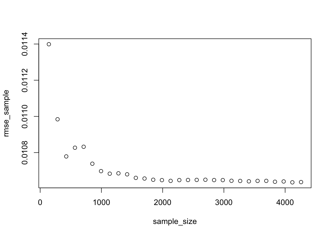
plot(sample_size,Rsq_sample)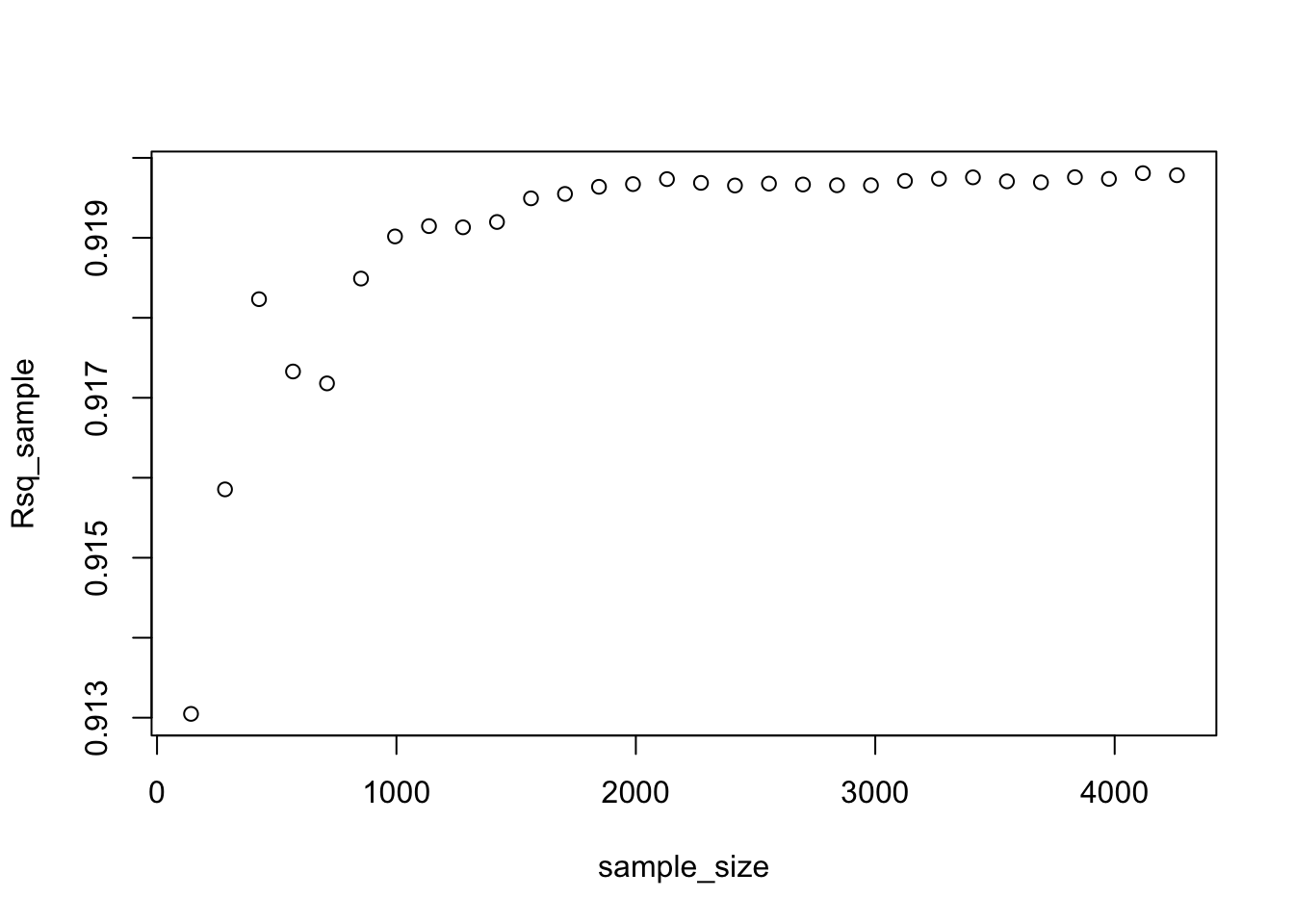
Q6 Analysis on learning curves
- When looking at the RMSE and R squared graphs, we can see that the RMSE decreases and the R squared increases a lot more before reaching the sample size of 2,000.
- This means that we would need approximately 2,000 in our sample size in order to estimate model 3 reliably. Once we reach this sample size, we can reduce the prediction error by changing the variables in our model (feature engineering), but not increasing sample size.
Regularization using LASSO regression
If we are in the region of the learning curve where we do not have enough data, one option is to use a regularization method such as LASSO.
Let’s try to estimate a large and complicated model (many interactions and polynomials) on a small training dataset using OLS regression and hold-out validation method.
#split the data in testing and training. The training test is really small.
set.seed(1234)
train_test_split <- initial_split(lc_clean, prop = 0.01)
training <- training(train_test_split)
testing <- testing(train_test_split)

model_lm<-lm(int_rate ~ poly(loan_amnt,3) + term+ dti + annual_inc + grade +grade:poly(loan_amnt,3):term +poly(loan_amnt,3):term +grade:term, training)
predictions <- predict(model_lm,testing)

# Model prediction performance
data.frame(
  RMSE = RMSE(predictions, testing$int_rate),
  Rsquare = R2(predictions, testing$int_rate)
)| RMSE | Rsquare |
|---|---|
| 0.0123 | 0.891 |
Not surprisingly this model does not perform well – as we knew form the learning curves we constructed for a simpler model we need a lot more data to estimate this model reliably. Try running it again with different seeds. The model’s performance tends to be sensitive to the choice of the training set.
LASSO regression offers one solution – it extends the OLS regression by penalizing the model for setting any coefficient estimate to a value that is different from zero. The penalty is proportional to a parameter lambda. This parameter cannot be estimated directly (and for this reason sometimes it is referred to as hyperparameter). lambda will be selected through k-fold cross validation so as to provide the best out-of-sample performance. As a result of the LASSO procedure, only those features that are more strongly associated with the outcome will have non-zero coefficient estimates and the estimated model will be less sensitive to the training set. Sometimes LASSO regression is referred to as regularization.
# we will look for the optimal lambda in this sequence (we will try 1000 different lambdas)
lambda_seq <- seq(0, 0.01, length = 1000)

# lasso regression using k-fold cross validation to select the best lambda

lasso <- train(
 int_rate ~ poly(loan_amnt,3) + term+ dti + annual_inc + grade +grade:poly(loan_amnt,3):term +poly(loan_amnt,3):term +grade:term,
 data = training,
 method = "glmnet",
  preProc = c("center", "scale"), #This option standardizes the data before running the LASSO regression
  trControl = control,
  tuneGrid = expand.grid(alpha = 1, lambda = lambda_seq) #alpha=1 specifies to run a LASSO regression. If alpha=0 the model would run ridge regression.
  )
## + Fold01: alpha=1, lambda=0.01
## - Fold01: alpha=1, lambda=0.01
## + Fold02: alpha=1, lambda=0.01
## - Fold02: alpha=1, lambda=0.01
## + Fold03: alpha=1, lambda=0.01
## - Fold03: alpha=1, lambda=0.01
## + Fold04: alpha=1, lambda=0.01
## - Fold04: alpha=1, lambda=0.01
## + Fold05: alpha=1, lambda=0.01
## - Fold05: alpha=1, lambda=0.01
## + Fold06: alpha=1, lambda=0.01
## - Fold06: alpha=1, lambda=0.01
## + Fold07: alpha=1, lambda=0.01
## - Fold07: alpha=1, lambda=0.01
## + Fold08: alpha=1, lambda=0.01
## - Fold08: alpha=1, lambda=0.01
## + Fold09: alpha=1, lambda=0.01
## - Fold09: alpha=1, lambda=0.01
## + Fold10: alpha=1, lambda=0.01
## - Fold10: alpha=1, lambda=0.01
## Aggregating results
## Selecting tuning parameters
## Fitting alpha = 1, lambda = 0.00032 on full training set# Model coefficients
coef(lasso$finalModel, lasso$bestTune$lambda)## 58 x 1 sparse Matrix of class "dgCMatrix"
## s1
## (Intercept) 1.211648e-01
## poly(loan_amnt, 3)1 8.147846e-04
## poly(loan_amnt, 3)2 .
## poly(loan_amnt, 3)3 2.318037e-04
## term60 1.315642e-03
## dti 4.468570e-04
## annual_inc .
## gradeB 1.689641e-02
## gradeC 2.336358e-02
## gradeD 2.495146e-02
## gradeE 2.491406e-02
## gradeF 1.898605e-02
## gradeG 1.746858e-02
## poly(loan_amnt, 3)1:term60 .
## poly(loan_amnt, 3)2:term60 .
## poly(loan_amnt, 3)3:term60 .
## term60:gradeB -8.625465e-04
## term60:gradeC .
## term60:gradeD 5.599650e-04
## term60:gradeE 1.733082e-03
## term60:gradeF 6.810212e-04
## term60:gradeG 1.610131e-03
## poly(loan_amnt, 3)1:term36:gradeB .
## poly(loan_amnt, 3)2:term36:gradeB .
## poly(loan_amnt, 3)3:term36:gradeB 4.427114e-04
## poly(loan_amnt, 3)1:term60:gradeB .
## poly(loan_amnt, 3)2:term60:gradeB 4.701917e-04
## poly(loan_amnt, 3)3:term60:gradeB .
## poly(loan_amnt, 3)1:term36:gradeC .
## poly(loan_amnt, 3)2:term36:gradeC 3.455465e-04
## poly(loan_amnt, 3)3:term36:gradeC -2.604887e-04
## poly(loan_amnt, 3)1:term60:gradeC .
## poly(loan_amnt, 3)2:term60:gradeC .
## poly(loan_amnt, 3)3:term60:gradeC -3.559988e-04
## poly(loan_amnt, 3)1:term36:gradeD .
## poly(loan_amnt, 3)2:term36:gradeD 5.728226e-04
## poly(loan_amnt, 3)3:term36:gradeD 2.996661e-04
## poly(loan_amnt, 3)1:term60:gradeD .
## poly(loan_amnt, 3)2:term60:gradeD .
## poly(loan_amnt, 3)3:term60:gradeD -5.402934e-05
## poly(loan_amnt, 3)1:term36:gradeE .
## poly(loan_amnt, 3)2:term36:gradeE .
## poly(loan_amnt, 3)3:term36:gradeE .
## poly(loan_amnt, 3)1:term60:gradeE .
## poly(loan_amnt, 3)2:term60:gradeE .
## poly(loan_amnt, 3)3:term60:gradeE -4.702642e-04
## poly(loan_amnt, 3)1:term36:gradeF .
## poly(loan_amnt, 3)2:term36:gradeF .
## poly(loan_amnt, 3)3:term36:gradeF .
## poly(loan_amnt, 3)1:term60:gradeF .
## poly(loan_amnt, 3)2:term60:gradeF .
## poly(loan_amnt, 3)3:term60:gradeF 1.398907e-03
## poly(loan_amnt, 3)1:term36:gradeG .
## poly(loan_amnt, 3)2:term36:gradeG .
## poly(loan_amnt, 3)3:term36:gradeG .
## poly(loan_amnt, 3)1:term60:gradeG .
## poly(loan_amnt, 3)2:term60:gradeG 4.631181e-04
## poly(loan_amnt, 3)3:term60:gradeG .# Best lambda
lasso$bestTune$lambda## [1] 0.0003203203# Count of how many coefficients are greater than zero and how many are equal to zero
sum(coef(lasso$finalModel, lasso$bestTune$lambda)!=0)## [1] 27sum(coef(lasso$finalModel, lasso$bestTune$lambda)==0)## [1] 31# Make predictions
predictions <- predict(lasso,testing)
# Model prediction performance
data.frame(
RMSE = RMSE(predictions, testing$int_rate),
Rsquare = R2(predictions, testing$int_rate)
)| RMSE | Rsquare |
|---|---|
| 0.0108 | 0.917 |
Q7 Comparison between OLS regression and LASSO
- Which model performs best out of sample, OLS regression or LASSO? Why?
- By comparing RMSE and LASSO, we can see LASSO performs better than OLS regression. The R square value increases by almost 0.03.
- What value of lambda offers best performance? Is this sensitive to the random seed? Why?
- The model performs best with lambda equals to 0.00038. This number is sensitive to the random seed because the lamda changes with different random seeds.
- How many coefficients are zero and how many are non-zero in the LASSO model of best fit? Is number of zero (or non-zero) coefficients sensitive on the random seed? Why?
- 26 coefficients are zero and 32 are non-zero. It is also sensitive to the random seed. We got different numbers with random seed of 4 and 5.
- Why is it important to standardize continuous variables before running LASSO?
- Because we have a penalty on the absolute values of coefficients. With different scales of continuous variables, the levels of coefficients can be very different, which introduces imbanlance of importance of variables.
Using Time Information
Let’s try to further improve the model’s predictive performance. So far we have not used any time series information. Effectively, all things being equal, our prediction for the interest rate of a loan given in 2009 would be the same as that of a loan given in 2011. We do not think it a good assumption and we are now taking into consideration the time series information to fix this in our previous models.
First, we investigate graphically whether there are any time trends in the interest rates. (Note that the variable “issue_d” only has information on the month the loan was awarded but not the exact date.) We want to use this to improve the model by tring controlling for time in a linear fashion (i.e., a linear time trend) and controlling for time as quarter-year dummies (this is a method to capture non-linear effects of time – we assume that the impact of time doesn’t change within a quarter but it can chance from quarter to quarter). Finally, we checked if time affect loans of different grades differently.
#linear time trend (add code below)
ggplot(lc_clean, aes(x=issue_d, y=int_rate))+
  geom_point(size=0.1)+
  geom_smooth(method = "lm", se=FALSE)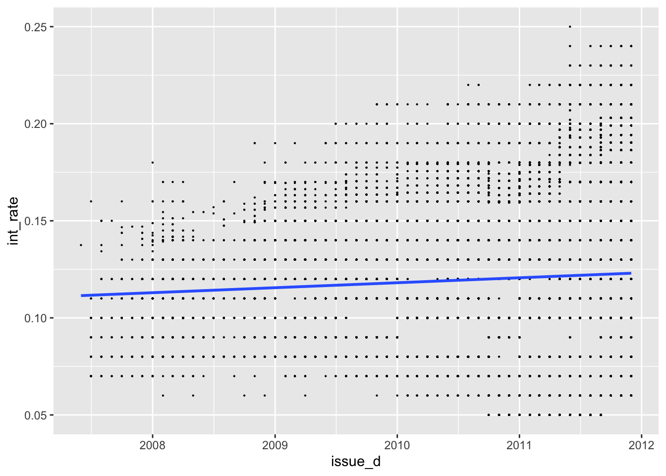
#linear time trend by grade (add code below)
ggplot(lc_clean, aes(x=issue_d, y=int_rate, color=grade))+
  geom_point(size=0.1)+
  geom_smooth(method = "lm", se=FALSE)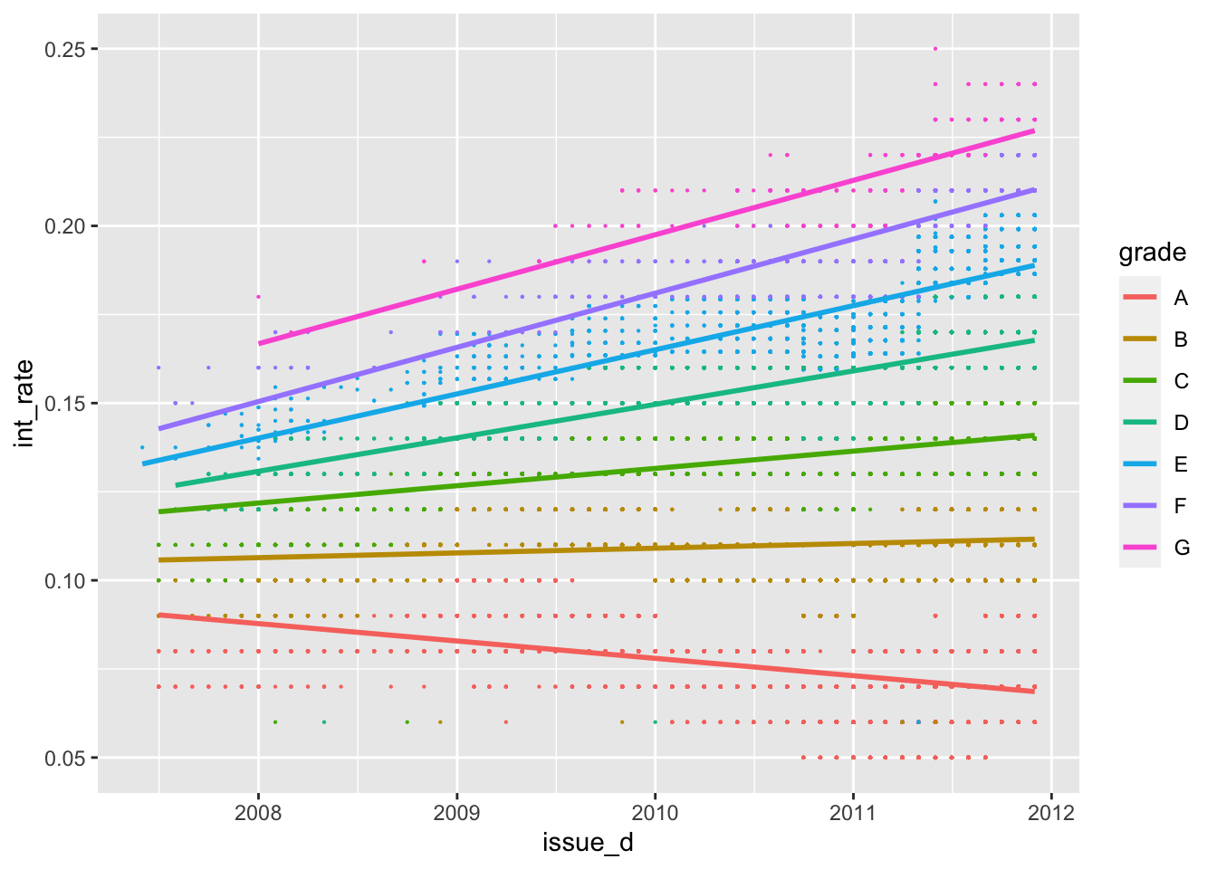
#Train models using OLS regression and k-fold cross-validation
#The first model has some explanatory variables and a linear time trend

time1<-train(
  int_rate ~ loan_amnt*grade + term +dti + quartiles_annual_inc + issue_d , #fill your variables here "+ issue_d"
  lc_clean,
  method = "lm",
  trControl = control)
## + Fold01: intercept=TRUE
## - Fold01: intercept=TRUE
## + Fold02: intercept=TRUE
## - Fold02: intercept=TRUE
## + Fold03: intercept=TRUE
## - Fold03: intercept=TRUE
## + Fold04: intercept=TRUE
## - Fold04: intercept=TRUE
## + Fold05: intercept=TRUE
## - Fold05: intercept=TRUE
## + Fold06: intercept=TRUE
## - Fold06: intercept=TRUE
## + Fold07: intercept=TRUE
## - Fold07: intercept=TRUE
## + Fold08: intercept=TRUE
## - Fold08: intercept=TRUE
## + Fold09: intercept=TRUE
## - Fold09: intercept=TRUE
## + Fold10: intercept=TRUE
## - Fold10: intercept=TRUE
## Aggregating results
## Fitting final model on full training setsummary(time1)##
## Call:
## lm(formula = .outcome ~ ., data = dat)
##
## Residuals:
## Min 1Q Median 3Q Max
## -0.118983 -0.006602 -0.000730 0.006935 0.036319
##
## Coefficients:
## Estimate Std. Error t value Pr(>|t|)
## (Intercept) -2.492e-02 2.512e-03 -9.921 < 2e-16 ***
## loan_amnt 1.008e-07 2.014e-08 5.001 5.71e-07 ***
## gradeB 3.607e-02 2.681e-04 134.564 < 2e-16 ***
## gradeC 6.244e-02 2.934e-04 212.772 < 2e-16 ***
## gradeD 8.127e-02 3.419e-04 237.674 < 2e-16 ***
## gradeE 9.727e-02 4.542e-04 214.134 < 2e-16 ***
## gradeF 1.152e-01 7.591e-04 151.828 < 2e-16 ***
## gradeG 1.336e-01 1.521e-03 87.854 < 2e-16 ***
## term60 2.238e-03 1.453e-04 15.400 < 2e-16 ***
## dti 8.506e-06 8.133e-06 1.046 0.295631
## quartiles_annual_inc2 -2.541e-04 1.518e-04 -1.674 0.094150 .
## quartiles_annual_inc3 -4.275e-04 1.560e-04 -2.740 0.006139 **
## quartiles_annual_inc4 -5.694e-04 1.660e-04 -3.430 0.000603 ***
## issue_d 6.542e-06 1.690e-07 38.700 < 2e-16 ***
## `loan_amnt:gradeB` -8.054e-11 2.401e-08 -0.003 0.997323
## `loan_amnt:gradeC` -1.200e-07 2.574e-08 -4.661 3.15e-06 ***
## `loan_amnt:gradeD` 1.151e-07 2.747e-08 4.189 2.80e-05 ***
## `loan_amnt:gradeE` 2.459e-07 2.959e-08 8.311 < 2e-16 ***
## `loan_amnt:gradeF` 3.005e-07 4.057e-08 7.407 1.31e-13 ***
## `loan_amnt:gradeG` 1.599e-07 7.120e-08 2.246 0.024721 *
## ---
## Signif. codes: 0 '***' 0.001 '**' 0.01 '*' 0.05 '.' 0.1 ' ' 1
##
## Residual standard error: 0.01031 on 37849 degrees of freedom
## Multiple R-squared: 0.9234, Adjusted R-squared: 0.9234
## F-statistic: 2.403e+04 on 19 and 37849 DF, p-value: < 2.2e-16#The second model has a different linear time trend for each grade class
time2<-train(
int_rate ~ loan_amnt*grade + term +dti + quartiles_annual_inc + issue_d * grade, #fill your variables here
lc_clean,
method = "lm",
trControl = control
)## + Fold01: intercept=TRUE
## - Fold01: intercept=TRUE
## + Fold02: intercept=TRUE
## - Fold02: intercept=TRUE
## + Fold03: intercept=TRUE
## - Fold03: intercept=TRUE
## + Fold04: intercept=TRUE
## - Fold04: intercept=TRUE
## + Fold05: intercept=TRUE
## - Fold05: intercept=TRUE
## + Fold06: intercept=TRUE
## - Fold06: intercept=TRUE
## + Fold07: intercept=TRUE
## - Fold07: intercept=TRUE
## + Fold08: intercept=TRUE
## - Fold08: intercept=TRUE
## + Fold09: intercept=TRUE
## - Fold09: intercept=TRUE
## + Fold10: intercept=TRUE
## - Fold10: intercept=TRUE
## Aggregating results
## Fitting final model on full training setsummary(time2)##
## Call:
## lm(formula = .outcome ~ ., data = dat)
##
## Residuals:
## Min 1Q Median 3Q Max
## -0.120720 -0.006613 -0.000134 0.006753 0.030865
##
## Coefficients:
## Estimate Std. Error t value Pr(>|t|)
## (Intercept) 2.862e-01 4.357e-03 65.681 < 2e-16 ***
## loan_amnt 3.156e-07 1.786e-08 17.673 < 2e-16 ***
## gradeB -2.298e-01 5.808e-03 -39.573 < 2e-16 ***
## gradeC -3.541e-01 6.178e-03 -57.315 < 2e-16 ***
## gradeD -5.147e-01 7.197e-03 -71.510 < 2e-16 ***
## gradeE -6.134e-01 9.904e-03 -61.935 < 2e-16 ***
## gradeF -7.098e-01 1.612e-02 -44.042 < 2e-16 ***
## gradeG -7.102e-01 3.314e-02 -21.432 < 2e-16 ***
## term60 -6.331e-04 1.304e-04 -4.856 1.20e-06 ***
## dti 5.407e-05 7.148e-06 7.564 4.00e-14 ***
## quartiles_annual_inc2 -2.976e-04 1.332e-04 -2.234 0.02547 *
## quartiles_annual_inc3 -3.926e-04 1.369e-04 -2.869 0.00412 **
## quartiles_annual_inc4 -5.857e-04 1.456e-04 -4.022 5.79e-05 ***
## issue_d -1.443e-05 2.935e-07 -49.179 < 2e-16 ***
## `loan_amnt:gradeB` -1.560e-07 2.122e-08 -7.352 1.99e-13 ***
## `loan_amnt:gradeC` -3.231e-07 2.283e-08 -14.154 < 2e-16 ***
## `loan_amnt:gradeD` -1.771e-07 2.435e-08 -7.276 3.50e-13 ***
## `loan_amnt:gradeE` -1.725e-07 2.658e-08 -6.489 8.76e-11 ***
## `loan_amnt:gradeF` -1.865e-07 3.677e-08 -5.072 3.95e-07 ***
## `loan_amnt:gradeG` -2.944e-07 6.439e-08 -4.572 4.85e-06 ***
## `gradeB:issue_d` 1.791e-05 3.903e-07 45.877 < 2e-16 ***
## `gradeC:issue_d` 2.807e-05 4.165e-07 67.402 < 2e-16 ***
## `gradeD:issue_d` 4.019e-05 4.849e-07 82.884 < 2e-16 ***
## `gradeE:issue_d` 4.799e-05 6.679e-07 71.852 < 2e-16 ***
## `gradeF:issue_d` 5.568e-05 1.085e-06 51.309 < 2e-16 ***
## `gradeG:issue_d` 5.695e-05 2.230e-06 25.541 < 2e-16 ***
## ---
## Signif. codes: 0 '***' 0.001 '**' 0.01 '*' 0.05 '.' 0.1 ' ' 1
##
## Residual standard error: 0.009048 on 37843 degrees of freedom
## Multiple R-squared: 0.9411, Adjusted R-squared: 0.9411
## F-statistic: 2.418e+04 on 25 and 37843 DF, p-value: < 2.2e-16#Change the time trend to a quarter dummy variables.
#zoo::as.yearqrt() creates quarter dummies
lc_clean_quarter<-lc_clean %>%
mutate(yq = as.factor(as.yearqtr(lc_clean$issue_d, format = "%Y-%m-%d")))
time3<-train(
int_rate ~ loan_amnt*grade + term +dti + quartiles_annual_inc + yq,#fill your variables here
lc_clean_quarter,
method = "lm",
trControl = control
)## + Fold01: intercept=TRUE
## - Fold01: intercept=TRUE
## + Fold02: intercept=TRUE
## - Fold02: intercept=TRUE
## + Fold03: intercept=TRUE
## - Fold03: intercept=TRUE
## + Fold04: intercept=TRUE
## - Fold04: intercept=TRUE
## + Fold05: intercept=TRUE
## - Fold05: intercept=TRUE
## + Fold06: intercept=TRUE
## - Fold06: intercept=TRUE
## + Fold07: intercept=TRUE
## - Fold07: intercept=TRUE
## + Fold08: intercept=TRUE
## - Fold08: intercept=TRUE
## + Fold09: intercept=TRUE
## - Fold09: intercept=TRUE
## + Fold10: intercept=TRUE
## - Fold10: intercept=TRUE
## Aggregating results
## Fitting final model on full training setsummary(time3)##
## Call:
## lm(formula = .outcome ~ ., data = dat)
##
## Residuals:
## Min 1Q Median 3Q Max
## -0.116112 -0.005421 -0.000205 0.005814 0.037669
##
## Coefficients:
## Estimate Std. Error t value Pr(>|t|)
## (Intercept) 3.826e-02 9.075e-03 4.215 2.50e-05 ***
## loan_amnt 1.089e-07 1.777e-08 6.127 9.02e-10 ***
## gradeB 3.657e-02 2.359e-04 155.008 < 2e-16 ***
## gradeC 6.248e-02 2.584e-04 241.762 < 2e-16 ***
## gradeD 8.095e-02 3.011e-04 268.891 < 2e-16 ***
## gradeE 9.699e-02 4.000e-04 242.508 < 2e-16 ***
## gradeF 1.154e-01 6.679e-04 172.748 < 2e-16 ***
## gradeG 1.338e-01 1.338e-03 99.989 < 2e-16 ***
## term60 4.576e-03 1.311e-04 34.916 < 2e-16 ***
## dti 5.287e-06 7.157e-06 0.739 0.460068
## quartiles_annual_inc2 -2.258e-04 1.336e-04 -1.690 0.090965 .
## quartiles_annual_inc3 -3.008e-04 1.373e-04 -2.191 0.028469 *
## quartiles_annual_inc4 -2.185e-04 1.462e-04 -1.495 0.134997
## `yq2007 Q3` 1.931e-02 9.136e-03 2.113 0.034581 *
## `yq2007 Q4` 1.486e-02 9.103e-03 1.632 0.102672
## `yq2008 Q1` 2.129e-02 9.082e-03 2.345 0.019051 *
## `yq2008 Q2` 2.292e-02 9.090e-03 2.522 0.011677 *
## `yq2008 Q3` 2.407e-02 9.100e-03 2.645 0.008161 **
## `yq2008 Q4` 3.201e-02 9.083e-03 3.525 0.000425 ***
## `yq2009 Q1` 3.619e-02 9.079e-03 3.986 6.74e-05 ***
## `yq2009 Q2` 3.803e-02 9.078e-03 4.189 2.80e-05 ***
## `yq2009 Q3` 3.957e-02 9.077e-03 4.359 1.31e-05 ***
## `yq2009 Q4` 3.981e-02 9.076e-03 4.386 1.16e-05 ***
## `yq2010 Q1` 3.480e-02 9.076e-03 3.834 0.000126 ***
## `yq2010 Q2` 3.355e-02 9.075e-03 3.697 0.000219 ***
## `yq2010 Q3` 3.464e-02 9.075e-03 3.817 0.000135 ***
## `yq2010 Q4` 2.592e-02 9.075e-03 2.856 0.004290 **
## `yq2011 Q1` 2.805e-02 9.075e-03 3.091 0.001996 **
## `yq2011 Q2` 3.321e-02 9.075e-03 3.660 0.000253 ***
## `yq2011 Q3` 3.561e-02 9.074e-03 3.925 8.70e-05 ***
## `yq2011 Q4` 4.184e-02 9.074e-03 4.611 4.02e-06 ***
## `loan_amnt:gradeB` -1.076e-07 2.117e-08 -5.083 3.73e-07 ***
## `loan_amnt:gradeC` -2.140e-07 2.271e-08 -9.421 < 2e-16 ***
## `loan_amnt:gradeD` 5.910e-08 2.422e-08 2.440 0.014700 *
## `loan_amnt:gradeE` 1.812e-07 2.609e-08 6.943 3.89e-12 ***
## `loan_amnt:gradeF` 2.255e-07 3.573e-08 6.311 2.81e-10 ***
## `loan_amnt:gradeG` 1.121e-07 6.265e-08 1.789 0.073581 .
## ---
## Signif. codes: 0 '***' 0.001 '**' 0.01 '*' 0.05 '.' 0.1 ' ' 1
##
## Residual standard error: 0.00907 on 37832 degrees of freedom
## Multiple R-squared: 0.9408, Adjusted R-squared: 0.9408
## F-statistic: 1.671e+04 on 36 and 37832 DF, p-value: < 2.2e-16#We specify one quarter dummy variable for each grade. This is going to be a large model as there are 19 quarters x 7 grades = 133 quarter-grade dummies.
time4<-train(
int_rate ~ loan_amnt*grade + term +dti + quartiles_annual_inc + yq * grade, #fill your variables here
lc_clean_quarter,
method = "lm",
trControl = control
)## + Fold01: intercept=TRUE
## - Fold01: intercept=TRUE
## + Fold02: intercept=TRUE
## - Fold02: intercept=TRUE
## + Fold03: intercept=TRUE
## - Fold03: intercept=TRUE
## + Fold04: intercept=TRUE
## - Fold04: intercept=TRUE
## + Fold05: intercept=TRUE
## - Fold05: intercept=TRUE
## + Fold06: intercept=TRUE
## - Fold06: intercept=TRUE
## + Fold07: intercept=TRUE
## - Fold07: intercept=TRUE
## + Fold08: intercept=TRUE
## - Fold08: intercept=TRUE
## + Fold09: intercept=TRUE
## - Fold09: intercept=TRUE
## + Fold10: intercept=TRUE
## - Fold10: intercept=TRUE
## Aggregating results
## Fitting final model on full training setsummary(time4)##
## Call:
## lm(formula = .outcome ~ ., data = dat)
##
## Residuals:
## Min 1Q Median 3Q Max
## -0.120445 -0.004941 0.000306 0.004671 0.034212
##
## Coefficients: (11 not defined because of singularities)
## Estimate Std. Error t value Pr(>|t|)
## (Intercept) 1.858e-02 7.578e-03 2.451 0.014248 *
## loan_amnt 3.008e-07 1.510e-08 19.922 < 2e-16 ***
## gradeB 4.305e-02 3.193e-04 134.841 < 2e-16 ***
## gradeC 6.974e-02 3.622e-04 192.538 < 2e-16 ***
## gradeD 9.702e-02 4.189e-04 231.621 < 2e-16 ***
## gradeE 1.177e-01 5.380e-04 218.715 < 2e-16 ***
## gradeF 1.390e-01 8.637e-04 160.926 < 2e-16 ***
## gradeG 1.603e-01 1.800e-03 89.015 < 2e-16 ***
## term60 1.727e-03 1.131e-04 15.276 < 2e-16 ***
## dti 4.804e-05 5.991e-06 8.017 1.11e-15 ***
## quartiles_annual_inc2 -2.415e-04 1.116e-04 -2.165 0.030375 *
## quartiles_annual_inc3 -2.668e-04 1.146e-04 -2.327 0.019978 *
## quartiles_annual_inc4 -1.833e-04 1.221e-04 -1.501 0.133291
## `yq2007 Q3` 5.495e-02 7.722e-03 7.116 1.13e-12 ***
## `yq2007 Q4` 5.596e-02 7.711e-03 7.257 4.03e-13 ***
## `yq2008 Q1` 5.958e-02 7.616e-03 7.823 5.27e-15 ***
## `yq2008 Q2` 6.104e-02 7.651e-03 7.978 1.53e-15 ***
## `yq2008 Q3` 6.042e-02 7.687e-03 7.860 3.96e-15 ***
## `yq2008 Q4` 6.682e-02 7.616e-03 8.773 < 2e-16 ***
## `yq2009 Q1` 6.852e-02 7.598e-03 9.017 < 2e-16 ***
## `yq2009 Q2` 6.798e-02 7.593e-03 8.953 < 2e-16 ***
## `yq2009 Q3` 6.614e-02 7.589e-03 8.715 < 2e-16 ***
## `yq2009 Q4` 6.414e-02 7.587e-03 8.454 < 2e-16 ***
## `yq2010 Q1` 5.714e-02 7.586e-03 7.532 5.10e-14 ***
## `yq2010 Q2` 5.506e-02 7.583e-03 7.260 3.93e-13 ***
## `yq2010 Q3` 5.502e-02 7.583e-03 7.256 4.08e-13 ***
## `yq2010 Q4` 4.396e-02 7.581e-03 5.799 6.73e-09 ***
## `yq2011 Q1` 4.584e-02 7.580e-03 6.047 1.49e-09 ***
## `yq2011 Q2` 4.672e-02 7.580e-03 6.164 7.16e-10 ***
## `yq2011 Q3` 4.691e-02 7.579e-03 6.189 6.10e-10 ***
## `yq2011 Q4` 5.391e-02 7.575e-03 7.117 1.13e-12 ***
## `loan_amnt:gradeB` -2.450e-07 1.794e-08 -13.659 < 2e-16 ***
## `loan_amnt:gradeC` -3.703e-07 1.928e-08 -19.214 < 2e-16 ***
## `loan_amnt:gradeD` -2.118e-07 2.056e-08 -10.300 < 2e-16 ***
## `loan_amnt:gradeE` -2.256e-07 2.255e-08 -10.003 < 2e-16 ***
## `loan_amnt:gradeF` -2.504e-07 3.154e-08 -7.938 2.12e-15 ***
## `loan_amnt:gradeG` -3.434e-07 5.653e-08 -6.075 1.25e-09 ***
## `gradeB:yq2007 Q3` -2.304e-02 2.299e-03 -10.020 < 2e-16 ***
## `gradeC:yq2007 Q3` -3.562e-02 2.423e-03 -14.697 < 2e-16 ***
## `gradeD:yq2007 Q3` -5.146e-02 3.711e-03 -13.867 < 2e-16 ***
## `gradeE:yq2007 Q3` -5.699e-02 5.566e-03 -10.240 < 2e-16 ***
## `gradeF:yq2007 Q3` -6.132e-02 3.759e-03 -16.311 < 2e-16 ***
## `gradeG:yq2007 Q3` NA NA NA NA
## `gradeB:yq2007 Q4` -2.403e-02 1.948e-03 -12.339 < 2e-16 ***
## `gradeC:yq2007 Q4` -3.566e-02 1.799e-03 -19.823 < 2e-16 ***
## `gradeD:yq2007 Q4` -5.008e-02 2.070e-03 -24.198 < 2e-16 ***
## `gradeE:yq2007 Q4` -5.084e-02 2.722e-03 -18.675 < 2e-16 ***
## `gradeF:yq2007 Q4` -5.443e-02 7.719e-03 -7.051 1.81e-12 ***
## `gradeG:yq2007 Q4` NA NA NA NA
## `gradeB:yq2008 Q1` -2.290e-02 9.838e-04 -23.277 < 2e-16 ***
## `gradeC:yq2008 Q1` -3.337e-02 1.049e-03 -31.813 < 2e-16 ***
## `gradeD:yq2008 Q1` -4.551e-02 1.178e-03 -38.642 < 2e-16 ***
## `gradeE:yq2008 Q1` -5.324e-02 1.655e-03 -32.171 < 2e-16 ***
## `gradeF:yq2008 Q1` -5.634e-02 2.844e-03 -19.807 < 2e-16 ***
## `gradeG:yq2008 Q1` -6.318e-02 5.523e-03 -11.441 < 2e-16 ***
## `gradeB:yq2008 Q2` -2.276e-02 1.363e-03 -16.697 < 2e-16 ***
## `gradeC:yq2008 Q2` -3.374e-02 1.393e-03 -24.226 < 2e-16 ***
## `gradeD:yq2008 Q2` -4.729e-02 1.647e-03 -28.715 < 2e-16 ***
## `gradeE:yq2008 Q2` -5.146e-02 2.910e-03 -17.687 < 2e-16 ***
## `gradeF:yq2008 Q2` -5.826e-02 3.592e-03 -16.218 < 2e-16 ***
## `gradeG:yq2008 Q2` NA NA NA NA
## `gradeB:yq2008 Q3` -2.023e-02 1.740e-03 -11.630 < 2e-16 ***
## `gradeC:yq2008 Q3` -3.115e-02 1.668e-03 -18.670 < 2e-16 ***
## `gradeD:yq2008 Q3` -4.497e-02 2.101e-03 -21.409 < 2e-16 ***
## `gradeE:yq2008 Q3` -4.673e-02 3.008e-03 -15.535 < 2e-16 ***
## `gradeF:yq2008 Q3` -5.664e-02 4.071e-03 -13.911 < 2e-16 ***
## `gradeG:yq2008 Q3` NA NA NA NA
## `gradeB:yq2008 Q4` -1.845e-02 1.018e-03 -18.121 < 2e-16 ***
## `gradeC:yq2008 Q4` -3.049e-02 1.053e-03 -28.962 < 2e-16 ***
## `gradeD:yq2008 Q4` -4.384e-02 1.289e-03 -34.014 < 2e-16 ***
## `gradeE:yq2008 Q4` -4.913e-02 1.676e-03 -29.310 < 2e-16 ***
## `gradeF:yq2008 Q4` -5.307e-02 3.907e-03 -13.582 < 2e-16 ***
## `gradeG:yq2008 Q4` -5.526e-02 5.535e-03 -9.984 < 2e-16 ***
## `gradeB:yq2009 Q1` -1.310e-02 9.322e-04 -14.050 < 2e-16 ***
## `gradeC:yq2009 Q1` -2.475e-02 8.185e-04 -30.233 < 2e-16 ***
## `gradeD:yq2009 Q1` -4.049e-02 9.186e-04 -44.076 < 2e-16 ***
## `gradeE:yq2009 Q1` -4.419e-02 1.249e-03 -35.372 < 2e-16 ***
## `gradeF:yq2009 Q1` -4.824e-02 2.811e-03 -17.163 < 2e-16 ***
## `gradeG:yq2009 Q1` NA NA NA NA
## `gradeB:yq2009 Q2` -1.349e-02 7.243e-04 -18.624 < 2e-16 ***
## `gradeC:yq2009 Q2` -2.424e-02 7.533e-04 -32.185 < 2e-16 ***
## `gradeD:yq2009 Q2` -4.049e-02 9.255e-04 -43.747 < 2e-16 ***
## `gradeE:yq2009 Q2` -4.479e-02 1.311e-03 -34.162 < 2e-16 ***
## `gradeF:yq2009 Q2` -5.316e-02 2.409e-03 -22.065 < 2e-16 ***
## `gradeG:yq2009 Q2` -5.700e-02 4.104e-03 -13.889 < 2e-16 ***
## `gradeB:yq2009 Q3` -1.140e-02 6.336e-04 -18.000 < 2e-16 ***
## `gradeC:yq2009 Q3` -2.039e-02 6.928e-04 -29.427 < 2e-16 ***
## `gradeD:yq2009 Q3` -3.290e-02 8.752e-04 -37.590 < 2e-16 ***
## `gradeE:yq2009 Q3` -3.719e-02 1.131e-03 -32.871 < 2e-16 ***
## `gradeF:yq2009 Q3` -4.274e-02 1.862e-03 -22.957 < 2e-16 ***
## `gradeG:yq2009 Q3` -4.753e-02 3.162e-03 -15.030 < 2e-16 ***
## `gradeB:yq2009 Q4` -8.481e-03 5.660e-04 -14.985 < 2e-16 ***
## `gradeC:yq2009 Q4` -1.674e-02 6.161e-04 -27.177 < 2e-16 ***
## `gradeD:yq2009 Q4` -2.822e-02 7.048e-04 -40.033 < 2e-16 ***
## `gradeE:yq2009 Q4` -3.367e-02 1.108e-03 -30.401 < 2e-16 ***
## `gradeF:yq2009 Q4` -3.639e-02 1.717e-03 -21.187 < 2e-16 ***
## `gradeG:yq2009 Q4` -3.763e-02 2.556e-03 -14.720 < 2e-16 ***
## `gradeB:yq2010 Q1` -1.070e-02 5.403e-04 -19.806 < 2e-16 ***
## `gradeC:yq2010 Q1` -1.153e-02 6.006e-04 -19.199 < 2e-16 ***
## `gradeD:yq2010 Q1` -2.164e-02 6.843e-04 -31.628 < 2e-16 ***
## `gradeE:yq2010 Q1` -2.497e-02 1.015e-03 -24.593 < 2e-16 ***
## `gradeF:yq2010 Q1` -3.071e-02 1.794e-03 -17.116 < 2e-16 ***
## `gradeG:yq2010 Q1` -2.975e-02 3.106e-03 -9.580 < 2e-16 ***
## `gradeB:yq2010 Q2` -9.913e-03 4.801e-04 -20.649 < 2e-16 ***
## `gradeC:yq2010 Q2` -8.584e-03 5.269e-04 -16.293 < 2e-16 ***
## `gradeD:yq2010 Q2` -1.870e-02 5.940e-04 -31.487 < 2e-16 ***
## `gradeE:yq2010 Q2` -2.299e-02 7.790e-04 -29.507 < 2e-16 ***
## `gradeF:yq2010 Q2` -2.840e-02 1.314e-03 -21.617 < 2e-16 ***
## `gradeG:yq2010 Q2` -2.824e-02 2.662e-03 -10.611 < 2e-16 ***
## `gradeB:yq2010 Q3` -7.443e-03 4.609e-04 -16.149 < 2e-16 ***
## `gradeC:yq2010 Q3` -5.014e-03 5.055e-04 -9.918 < 2e-16 ***
## `gradeD:yq2010 Q3` -1.705e-02 5.669e-04 -30.074 < 2e-16 ***
## `gradeE:yq2010 Q3` -2.373e-02 6.796e-04 -34.922 < 2e-16 ***
## `gradeF:yq2010 Q3` -2.740e-02 1.094e-03 -25.037 < 2e-16 ***
## `gradeG:yq2010 Q3` -2.536e-02 1.880e-03 -13.488 < 2e-16 ***
## `gradeB:yq2010 Q4` -7.629e-03 4.269e-04 -17.872 < 2e-16 ***
## `gradeC:yq2010 Q4` -9.741e-04 4.811e-04 -2.025 0.042900 *
## `gradeD:yq2010 Q4` -1.265e-02 5.558e-04 -22.754 < 2e-16 ***
## `gradeE:yq2010 Q4` -1.655e-02 6.725e-04 -24.607 < 2e-16 ***
## `gradeF:yq2010 Q4` -1.942e-02 1.055e-03 -18.412 < 2e-16 ***
## `gradeG:yq2010 Q4` -1.928e-02 1.690e-03 -11.409 < 2e-16 ***
## `gradeB:yq2011 Q1` -5.823e-03 4.113e-04 -14.159 < 2e-16 ***
## `gradeC:yq2011 Q1` -2.384e-03 4.731e-04 -5.041 4.66e-07 ***
## `gradeD:yq2011 Q1` -1.072e-02 5.270e-04 -20.332 < 2e-16 ***
## `gradeE:yq2011 Q1` -1.575e-02 6.063e-04 -25.972 < 2e-16 ***
## `gradeF:yq2011 Q1` -1.818e-02 8.535e-04 -21.295 < 2e-16 ***
## `gradeG:yq2011 Q1` -2.123e-02 1.555e-03 -13.651 < 2e-16 ***
## `gradeB:yq2011 Q2` -1.318e-03 3.914e-04 -3.368 0.000759 ***
## `gradeC:yq2011 Q2` 3.869e-04 4.420e-04 0.875 0.381430
## `gradeD:yq2011 Q2` -4.212e-03 4.944e-04 -8.519 < 2e-16 ***
## `gradeE:yq2011 Q2` -5.559e-03 5.849e-04 -9.504 < 2e-16 ***
## `gradeF:yq2011 Q2` -5.157e-03 8.426e-04 -6.120 9.47e-10 ***
## `gradeG:yq2011 Q2` -1.097e-02 1.592e-03 -6.890 5.66e-12 ***
## `gradeB:yq2011 Q3` 1.318e-03 3.652e-04 3.609 0.000308 ***
## `gradeC:yq2011 Q3` 2.390e-03 4.221e-04 5.662 1.50e-08 ***
## `gradeD:yq2011 Q3` -3.556e-04 4.749e-04 -0.749 0.453964
## `gradeE:yq2011 Q3` 1.596e-03 5.763e-04 2.770 0.005611 **
## `gradeF:yq2011 Q3` 9.203e-04 8.587e-04 1.072 0.283847
## `gradeG:yq2011 Q3` -1.687e-03 1.643e-03 -1.027 0.304369
## `gradeB:yq2011 Q4` NA NA NA NA
## `gradeC:yq2011 Q4` NA NA NA NA
## `gradeD:yq2011 Q4` NA NA NA NA
## `gradeE:yq2011 Q4` NA NA NA NA
## `gradeF:yq2011 Q4` NA NA NA NA
## `gradeG:yq2011 Q4` NA NA NA NA
## ---
## Signif. codes: 0 '***' 0.001 '**' 0.01 '*' 0.05 '.' 0.1 ' ' 1
##
## Residual standard error: 0.007563 on 37735 degrees of freedom
## Multiple R-squared: 0.959, Adjusted R-squared: 0.9588
## F-statistic: 6628 on 133 and 37735 DF, p-value: < 2.2e-16data.frame(
time1$results$RMSE,
time2$results$RMSE,
time3$results$RMSE,
time4$results$RMSE)| time1.results.RMSE | time2.results.RMSE | time3.results.RMSE | time4.results.RMSE |
|---|---|---|---|
| 0.0103 | 0.00905 | 0.00908 | 0.00758 |
Q8 Prediction improvement by adding time information
- From the results of linear regressions, we find almost all the time related variables significant. Therefore, the interest rates do change over time.
- The predictions can be improved by adding quarter-year dummies. The RMSE has been improved from 0.0103 to 0.0076.
Using Bond Yields
One concern with using time trends for forecasting is that in order to make predictions for future loans we will need to project trends to the future. This is an extrapolation that may not be reasonable, especially if macroeconomic conditions in the future change. Furthermore, if we are using quarter-year dummies, it is not even possible to estimate the coefficient of these dummy variables for future quarters.
Instead, perhaps it’s better to find the reasons as to why different periods are different from one another. The csv file “MonthBondYields.csv” contains information on the yield of US Treasuries on the first day of each month. Can you use it to see if you can improve your predictions without using time dummies?
#load the data to memory as a dataframe
bond_prices<-readr::read_csv(here::here("data","MonthBondYields.csv"))

#make the date of the bond file comparable to the lending club dataset
#for some regional date/number (locale) settings this may not work. If it does try running the following line of code in the Console
#Sys.setlocale("LC_TIME","English")
bond_prices <- bond_prices %>%
  mutate(Date2=as.Date(paste("01",Date,sep="-"),"%d-%b-%y")) %>%
  select(-starts_with("X"))

#let's see what happened to bond yields over time. Lower bond yields mean the cost of borrowing has gone down.

bond_prices %>%
  ggplot(aes(x=Date2, y=Price))+
  geom_point(size=0.1, alpha=0.5)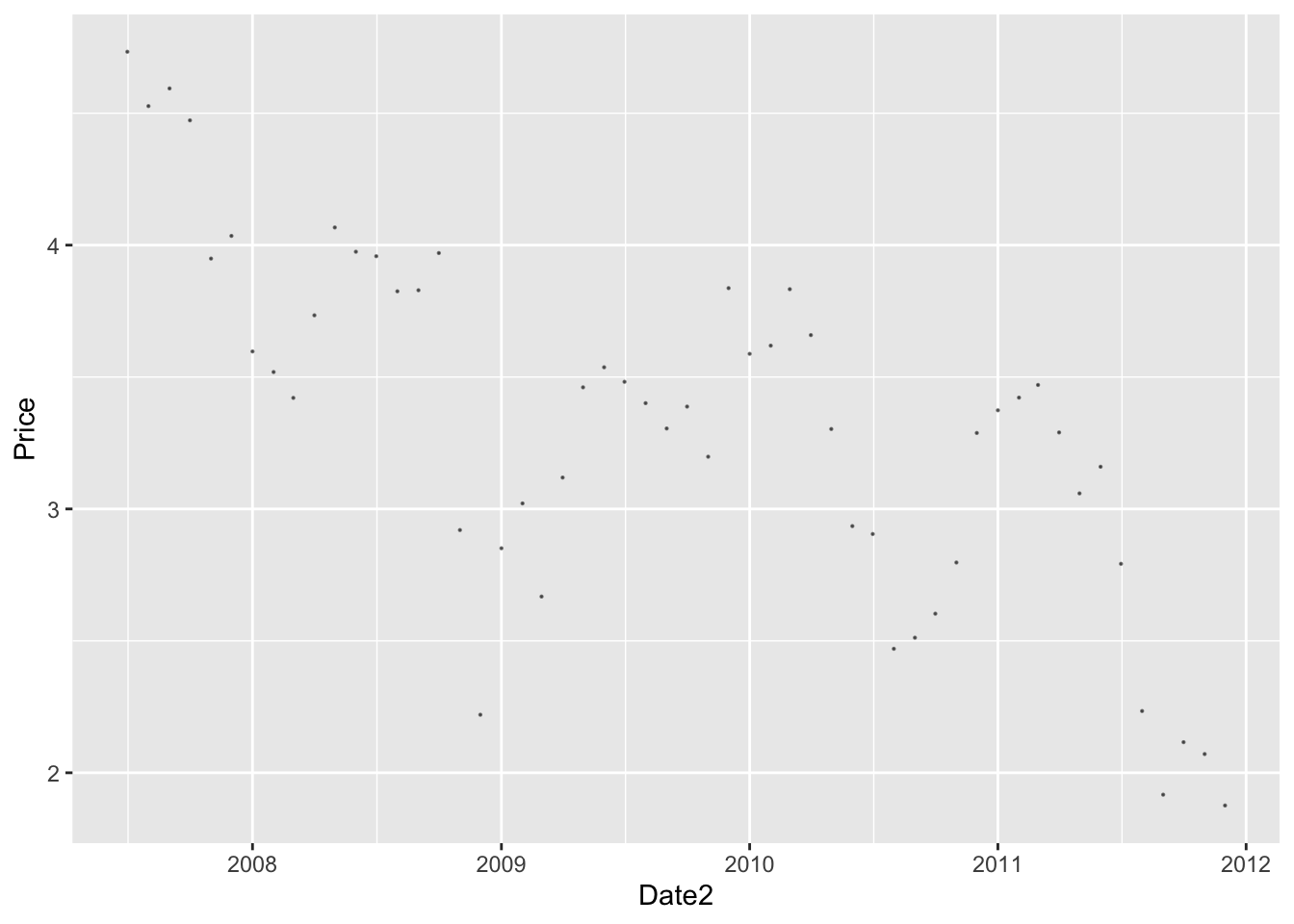
#join the data using a left join
lc_with_bonds <- lc_clean %>%
  mutate(yq = as.factor(as.yearqtr(lc_clean$issue_d, format = "%Y-%m-%d"))) %>%
  left_join(bond_prices, by = c("issue_d" = "Date2")) %>%
  arrange(issue_d) %>%
  filter(!is.na(Price)) #drop any observations where there re no bond prices available

# investigate graphically if there is a relationship
lc_with_bonds%>%
  ggplot(aes(x=int_rate, y=Price))+
  geom_point(size=0.1, alpha=0.5)+geom_smooth(method="lm")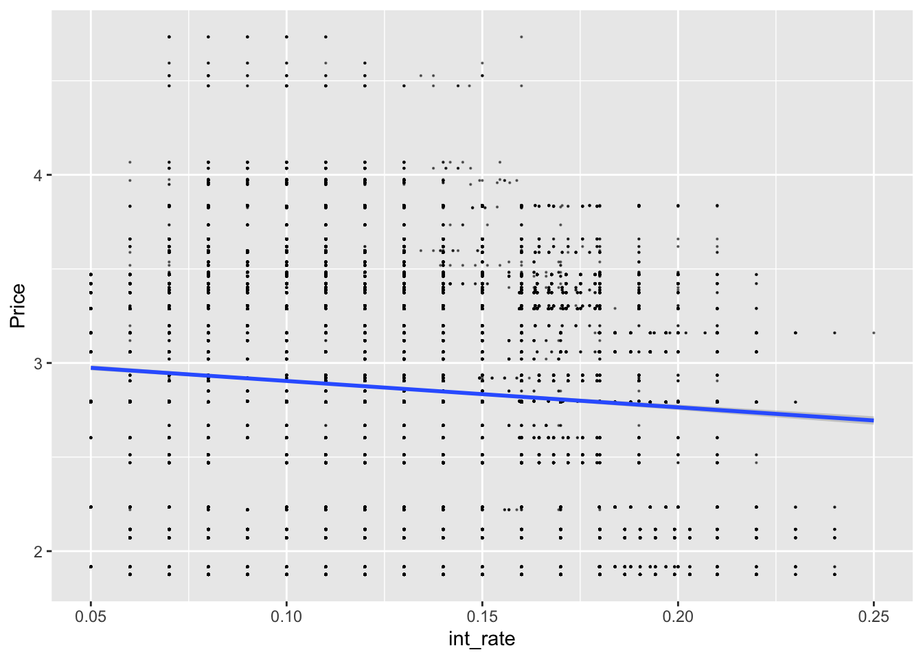
lc_with_bonds%>%
  ggplot(aes(x=int_rate, y=Price, color=grade))+
  geom_point(size=0.1, alpha=0.5)+
  geom_smooth(method="lm")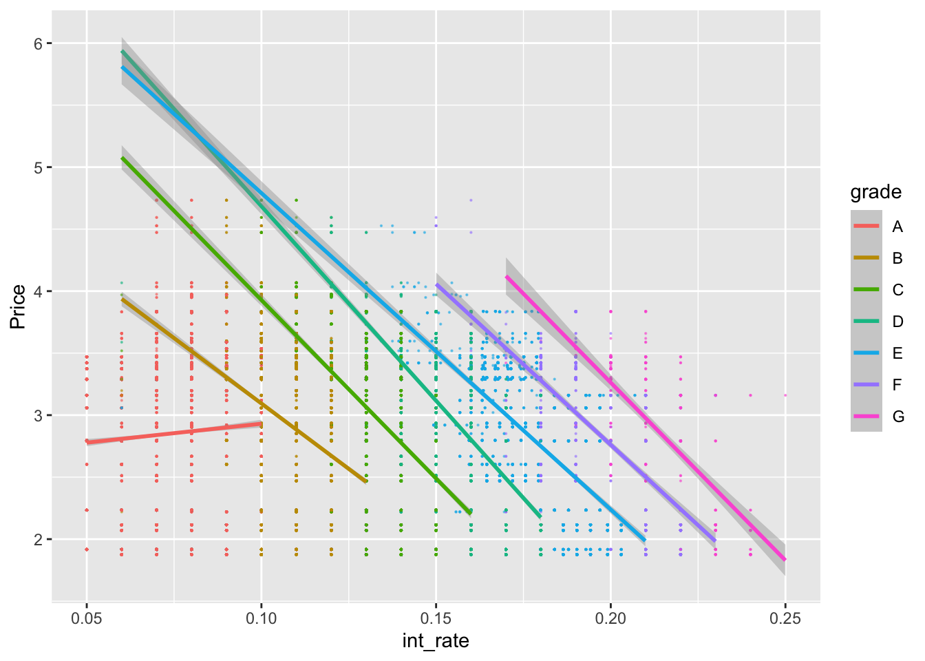
#let's train a model using the bond information
control <- trainControl (
    method="cv",
    number=10,
    verboseIter=TRUE)

plsFit<-train(
    int_rate ~  loan_amnt*grade + term +dti + Price * grade,
    lc_with_bonds,
    method = "lm",
    trControl = control
   )
## + Fold01: intercept=TRUE
## - Fold01: intercept=TRUE
## + Fold02: intercept=TRUE
## - Fold02: intercept=TRUE
## + Fold03: intercept=TRUE
## - Fold03: intercept=TRUE
## + Fold04: intercept=TRUE
## - Fold04: intercept=TRUE
## + Fold05: intercept=TRUE
## - Fold05: intercept=TRUE
## + Fold06: intercept=TRUE
## - Fold06: intercept=TRUE
## + Fold07: intercept=TRUE
## - Fold07: intercept=TRUE
## + Fold08: intercept=TRUE
## - Fold08: intercept=TRUE
## + Fold09: intercept=TRUE
## - Fold09: intercept=TRUE
## + Fold10: intercept=TRUE
## - Fold10: intercept=TRUE
## Aggregating results
## Fitting final model on full training setsummary(plsFit)##
## Call:
## lm(formula = .outcome ~ ., data = dat)
##
## Residuals:
## Min 1Q Median 3Q Max
## -0.117450 -0.005810 -0.000302 0.006494 0.040734
##
## Coefficients:
## Estimate Std. Error t value Pr(>|t|)
## (Intercept) 6.791e-02 5.361e-04 126.679 < 2e-16 ***
## loan_amnt 1.795e-07 1.863e-08 9.638 < 2e-16 ***
## gradeB 5.350e-02 6.990e-04 76.538 < 2e-16 ***
## gradeC 8.631e-02 7.843e-04 110.051 < 2e-16 ***
## gradeD 1.192e-01 8.941e-04 133.269 < 2e-16 ***
## gradeE 1.433e-01 1.167e-03 122.786 < 2e-16 ***
## gradeF 1.667e-01 1.791e-03 93.096 < 2e-16 ***
## gradeG 1.903e-01 3.456e-03 55.057 < 2e-16 ***
## term60 1.506e-03 1.323e-04 11.378 < 2e-16 ***
## dti 2.802e-05 7.453e-06 3.760 0.000171 ***
## Price 1.301e-03 1.626e-04 8.005 1.22e-15 ***
## `loan_amnt:gradeB` -9.477e-08 2.249e-08 -4.214 2.51e-05 ***
## `loan_amnt:gradeC` -2.195e-07 2.416e-08 -9.088 < 2e-16 ***
## `loan_amnt:gradeD` -1.987e-09 2.572e-08 -0.077 0.938417
## `loan_amnt:gradeE` 6.441e-08 2.787e-08 2.311 0.020827 *
## `loan_amnt:gradeF` 6.990e-08 3.840e-08 1.820 0.068693 .
## `loan_amnt:gradeG` -1.206e-07 6.770e-08 -1.781 0.074911 .
## `gradeB:Price` -5.774e-03 2.181e-04 -26.470 < 2e-16 ***
## `gradeC:Price` -8.000e-03 2.429e-04 -32.934 < 2e-16 ***
## `gradeD:Price` -1.274e-02 2.794e-04 -45.585 < 2e-16 ***
## `gradeE:Price` -1.527e-02 3.611e-04 -42.287 < 2e-16 ***
## `gradeF:Price` -1.667e-02 5.359e-04 -31.103 < 2e-16 ***
## `gradeG:Price` -1.780e-02 9.982e-04 -17.829 < 2e-16 ***
## ---
## Signif. codes: 0 '***' 0.001 '**' 0.01 '*' 0.05 '.' 0.1 ' ' 1
##
## Residual standard error: 0.009584 on 37845 degrees of freedom
## Multiple R-squared: 0.9339, Adjusted R-squared: 0.9339
## F-statistic: 2.43e+04 on 22 and 37845 DF, p-value: < 2.2e-16Q9 Explanatory power of bond yields
- We are using loan amount times grade,term, dti and Price times grade to predict the interest rates
- Yes, by adding bond yields to the model, the adjusted R square increased by 0.01, and the bond yields are significant on every grade.
- With increase in bond yield (price) by 1%, the interest rates on the loan increase by 0.13% on Grade A loans. As the grade decreases (A to G) the effect of bond yields (price) on the interest rate starts to become negative. This means that as treasury yields (price) increases, the effect on interest rates start to decrease.
Q10 Model Comparison
TestModel1<-train(
    int_rate ~  loan_amnt*grade + term +dti + Price * grade,
    lc_with_bonds,
    method = "lm",
    trControl = control
   )
## + Fold01: intercept=TRUE
## - Fold01: intercept=TRUE
## + Fold02: intercept=TRUE
## - Fold02: intercept=TRUE
## + Fold03: intercept=TRUE
## - Fold03: intercept=TRUE
## + Fold04: intercept=TRUE
## - Fold04: intercept=TRUE
## + Fold05: intercept=TRUE
## - Fold05: intercept=TRUE
## + Fold06: intercept=TRUE
## - Fold06: intercept=TRUE
## + Fold07: intercept=TRUE
## - Fold07: intercept=TRUE
## + Fold08: intercept=TRUE
## - Fold08: intercept=TRUE
## + Fold09: intercept=TRUE
## - Fold09: intercept=TRUE
## + Fold10: intercept=TRUE
## - Fold10: intercept=TRUE
## Aggregating results
## Fitting final model on full training setsummary(TestModel1)##
## Call:
## lm(formula = .outcome ~ ., data = dat)
##
## Residuals:
## Min 1Q Median 3Q Max
## -0.117450 -0.005810 -0.000302 0.006494 0.040734
##
## Coefficients:
## Estimate Std. Error t value Pr(>|t|)
## (Intercept) 6.791e-02 5.361e-04 126.679 < 2e-16 ***
## loan_amnt 1.795e-07 1.863e-08 9.638 < 2e-16 ***
## gradeB 5.350e-02 6.990e-04 76.538 < 2e-16 ***
## gradeC 8.631e-02 7.843e-04 110.051 < 2e-16 ***
## gradeD 1.192e-01 8.941e-04 133.269 < 2e-16 ***
## gradeE 1.433e-01 1.167e-03 122.786 < 2e-16 ***
## gradeF 1.667e-01 1.791e-03 93.096 < 2e-16 ***
## gradeG 1.903e-01 3.456e-03 55.057 < 2e-16 ***
## term60 1.506e-03 1.323e-04 11.378 < 2e-16 ***
## dti 2.802e-05 7.453e-06 3.760 0.000171 ***
## Price 1.301e-03 1.626e-04 8.005 1.22e-15 ***
## `loan_amnt:gradeB` -9.477e-08 2.249e-08 -4.214 2.51e-05 ***
## `loan_amnt:gradeC` -2.195e-07 2.416e-08 -9.088 < 2e-16 ***
## `loan_amnt:gradeD` -1.987e-09 2.572e-08 -0.077 0.938417
## `loan_amnt:gradeE` 6.441e-08 2.787e-08 2.311 0.020827 *
## `loan_amnt:gradeF` 6.990e-08 3.840e-08 1.820 0.068693 .
## `loan_amnt:gradeG` -1.206e-07 6.770e-08 -1.781 0.074911 .
## `gradeB:Price` -5.774e-03 2.181e-04 -26.470 < 2e-16 ***
## `gradeC:Price` -8.000e-03 2.429e-04 -32.934 < 2e-16 ***
## `gradeD:Price` -1.274e-02 2.794e-04 -45.585 < 2e-16 ***
## `gradeE:Price` -1.527e-02 3.611e-04 -42.287 < 2e-16 ***
## `gradeF:Price` -1.667e-02 5.359e-04 -31.103 < 2e-16 ***
## `gradeG:Price` -1.780e-02 9.982e-04 -17.829 < 2e-16 ***
## ---
## Signif. codes: 0 '***' 0.001 '**' 0.01 '*' 0.05 '.' 0.1 ' ' 1
##
## Residual standard error: 0.009584 on 37845 degrees of freedom
## Multiple R-squared: 0.9339, Adjusted R-squared: 0.9339
## F-statistic: 2.43e+04 on 22 and 37845 DF, p-value: < 2.2e-16# TestModel2<-train(
# int_rate ~ loan_amnt*grade + term +dti + Price * grade + quartiles_annual_inc + home_ownership + addr_state ,
# lc_with_bonds,
# method = "lm",
# trControl = control
# )
# summary(TestModel2)
#
# TestModel3<-train(
# int_rate ~ loan_amnt*grade + term +dti + Price * grade + quartiles_annual_inc + term*loan_amnt,
# lc_with_bonds,
# method = "lm",
# trControl = control
# )
# summary(TestModel3)We have tried different models by adding home ownership, loan purpose, delinq_2 years,quartiles_annual_income and term*loan_amt, and they have either decreased our R-squared or increased it very insignificantly. By adding more interaction terms and time information, the R^2 can be improved to 96% but it takes hours to run the model.
After several attempts to increase the performance of the model (RMSE, R^2) by adding additional variables, we consider TestModel1 is the best model. This is because the performance doesn’t improve significantly with more variables and TestModel1 is the least complex while with enough accuracy.
TestModel1 uses loam_amnt\(\times\)grade, term, dti, Price\(\times\)grade, quartiles_annual_inc to predict the interest rate. It achieves an R^2 of 0.934 and an RMSE of 0.009584. The model can be used for prediction and extrapolated into the future as we didn’t include any time dummy variables.
TestModel1 has a 95% confidence interval with a length of \(1.96\times0.009584\times 2=0.0375\).
Q11 Further improvements
Adding quarterly data on US CPI:
cpi <- readr::read_csv(here::here("data","ConsumerPriceIndex.csv")) %>%
  mutate(yq = as.factor(as.yearqtr(DATE, format = "%Y-%m-%d")))

lc_bonds_cpi <- lc_with_bonds %>%
  left_join(cpi, by = c("yq")) %>%
  arrange(issue_d) %>%
  filter(!is.na(CPALTT01USQ657N_NBD19600401)) #drop any observations where there re no bond prices available

# investigate graphically if there is a relationship
lc_bonds_cpi%>%
  ggplot(aes(x=CPALTT01USQ657N_NBD19600401))+
  geom_histogram()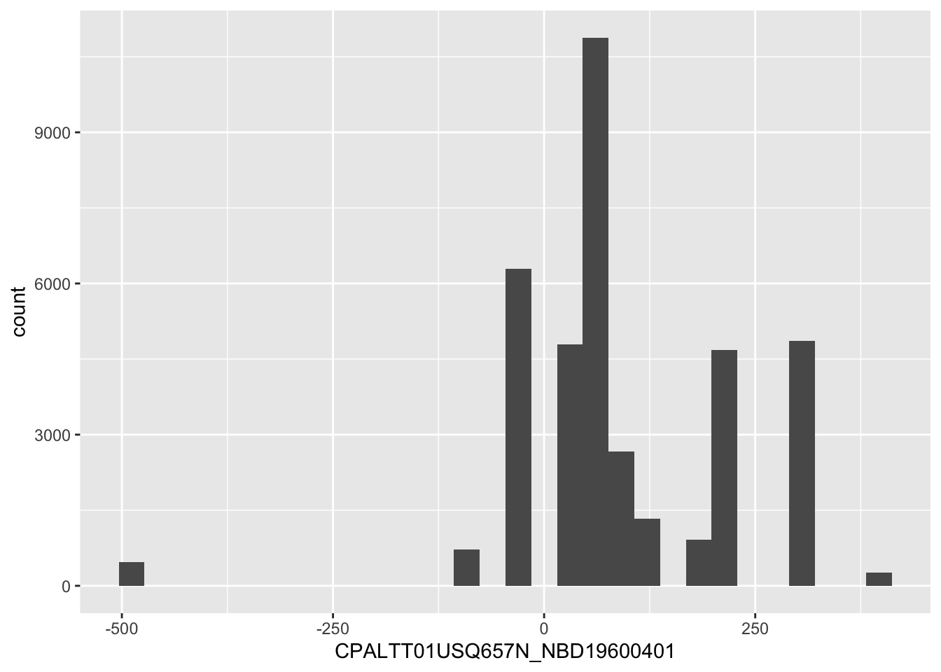
# investigate graphically if there is a relationship
lc_bonds_cpi%>%
  ggplot(aes(x=int_rate, y=CPALTT01USQ657N_NBD19600401))+
  geom_point(size=0.1, alpha=0.5)+
  geom_smooth(method="lm")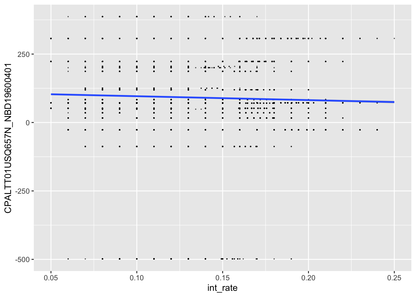
lc_bonds_cpi%>%
  ggplot(aes(x=int_rate, y=CPALTT01USQ657N_NBD19600401, color=grade))+
  geom_point(size=0.1, alpha=0.5)+
  geom_smooth(method="lm")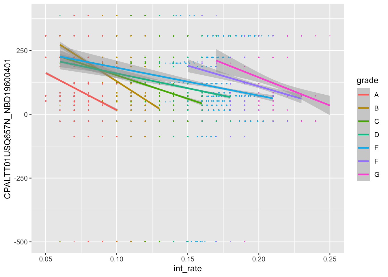
plsFit<-train(
    int_rate ~  loan_amnt*grade + term +dti +  Price*grade+ CPALTT01USQ657N_NBD19600401 * grade, #fill your variables here
    lc_bonds_cpi,
    method = "lm",
    trControl = control
   )
## + Fold01: intercept=TRUE
## - Fold01: intercept=TRUE
## + Fold02: intercept=TRUE
## - Fold02: intercept=TRUE
## + Fold03: intercept=TRUE
## - Fold03: intercept=TRUE
## + Fold04: intercept=TRUE
## - Fold04: intercept=TRUE
## + Fold05: intercept=TRUE
## - Fold05: intercept=TRUE
## + Fold06: intercept=TRUE
## - Fold06: intercept=TRUE
## + Fold07: intercept=TRUE
## - Fold07: intercept=TRUE
## + Fold08: intercept=TRUE
## - Fold08: intercept=TRUE
## + Fold09: intercept=TRUE
## - Fold09: intercept=TRUE
## + Fold10: intercept=TRUE
## - Fold10: intercept=TRUE
## Aggregating results
## Fitting final model on full training setsummary(plsFit)##
## Call:
## lm(formula = .outcome ~ ., data = dat)
##
## Residuals:
## Min 1Q Median 3Q Max
## -0.118658 -0.006044 0.000158 0.006133 0.036126
##
## Coefficients:
## Estimate Std. Error t value Pr(>|t|)
## (Intercept) 6.126e-02 5.479e-04 111.807 < 2e-16 ***
## loan_amnt 1.788e-07 1.802e-08 9.922 < 2e-16 ***
## gradeB 5.823e-02 7.151e-04 81.438 < 2e-16 ***
## gradeC 9.425e-02 8.014e-04 117.599 < 2e-16 ***
## gradeD 1.307e-01 9.211e-04 141.854 < 2e-16 ***
## gradeE 1.605e-01 1.253e-03 128.052 < 2e-16 ***
## gradeF 1.881e-01 1.998e-03 94.156 < 2e-16 ***
## gradeG 2.073e-01 3.733e-03 55.517 < 2e-16 ***
## term60 8.458e-04 1.316e-04 6.428 1.31e-10 ***
## dti 3.628e-05 7.218e-06 5.026 5.03e-07 ***
## Price 4.686e-03 1.810e-04 25.897 < 2e-16 ***
## CPALTT01USQ657N_NBD19600401 -3.294e-05 8.684e-07 -37.935 < 2e-16 ***
## `loan_amnt:gradeB` -8.482e-08 2.176e-08 -3.897 9.74e-05 ***
## `loan_amnt:gradeC` -2.087e-07 2.338e-08 -8.926 < 2e-16 ***
## `loan_amnt:gradeD` -9.708e-09 2.490e-08 -0.390 0.6966
## `loan_amnt:gradeE` 1.818e-08 2.708e-08 0.671 0.5021
## `loan_amnt:gradeF` 6.319e-09 3.744e-08 0.169 0.8660
## `loan_amnt:gradeG` -1.540e-07 6.578e-08 -2.342 0.0192 *
## `gradeB:Price` -8.189e-03 2.423e-04 -33.794 < 2e-16 ***
## `gradeC:Price` -1.200e-02 2.668e-04 -44.980 < 2e-16 ***
## `gradeD:Price` -1.837e-02 3.103e-04 -59.204 < 2e-16 ***
## `gradeE:Price` -2.315e-02 4.237e-04 -54.637 < 2e-16 ***
## `gradeF:Price` -2.646e-02 6.832e-04 -38.735 < 2e-16 ***
## `gradeG:Price` -2.564e-02 1.223e-03 -20.958 < 2e-16 ***
## `gradeB:CPALTT01USQ657N_NBD19600401` 2.277e-05 1.158e-06 19.662 < 2e-16 ***
## `gradeC:CPALTT01USQ657N_NBD19600401` 3.827e-05 1.232e-06 31.071 < 2e-16 ***
## `gradeD:CPALTT01USQ657N_NBD19600401` 5.315e-05 1.437e-06 36.997 < 2e-16 ***
## `gradeE:CPALTT01USQ657N_NBD19600401` 6.583e-05 1.870e-06 35.193 < 2e-16 ***
## `gradeF:CPALTT01USQ657N_NBD19600401` 7.705e-05 3.175e-06 24.266 < 2e-16 ***
## `gradeG:CPALTT01USQ657N_NBD19600401` 6.397e-05 5.445e-06 11.750 < 2e-16 ***
## ---
## Signif. codes: 0 '***' 0.001 '**' 0.01 '*' 0.05 '.' 0.1 ' ' 1
##
## Residual standard error: 0.009273 on 37838 degrees of freedom
## Multiple R-squared: 0.9381, Adjusted R-squared: 0.9381
## F-statistic: 1.978e+04 on 29 and 37838 DF, p-value: < 2.2e-16Analysis on additional data
- We would think that the additional data on inflation will make a difference because by adding both the bond yield and the inflation rate as variables to the model, it will give us a more accurate view on the real interest rate at the time.
- However, when running the model, we can see that the adjusted r-squared only increases by more than 0.4% to 93.81%. The model also has a lower RMSE, making the predictions more accurate.
Team members
- Alex Kubbinga
- Clara Moreno Sanchez
- Jean Huang
- Raghav Mehta
- Raina Doshi
- Yuan Gao