1. Load the data

fff = read_csv("F-F_Research_Data_Factors.CSV",skip = 2,n_max = 1146)
colnames(fff)[1] = "date"
data = read_csv("25_Portfolios_5x5.CSV",skip = 15,n_max = 1146)
colnames(data)[1] = "date"

operating = read_csv("Portfolios_Formed_on_OP.CSV",skip = 24,n_max = 702) %>% select(1,10:19)
colnames(operating) = paste(colnames(operating), "op", sep = "_")
colnames(operating)[1] = "date"
inv = read_csv("Portfolios_Formed_on_INV.CSV",skip = 17,n_max = 702) %>% select(1,10:19)
colnames(inv) = paste(colnames(inv), "inv", sep = "_")
colnames(inv)[1] = "date"
devidends = read_csv("Portfolios_Formed_on_D-P.CSV",skip = 19,n_max = 1134) %>% select(1,11:20)
colnames(devidends) = paste(colnames(devidends), "div", sep = "_")
colnames(devidends)[1] = "date"
momentum = read_csv("10_Portfolios_Prior_12_2.CSV",skip = 10,n_max = 1140)
colnames(momentum) = paste(colnames(momentum), "mom", sep = "_")
colnames(momentum)[1] = "date"

industry17 = read_csv("17_Industry_Portfolios.CSV",skip = 11,n_max = 1146)
colnames(industry17) = paste(colnames(industry17), "17", sep = "_")
colnames(industry17)[1] = "date"
industry30 = read_csv("30_Industry_Portfolios.CSV",skip = 11,n_max = 1146)
colnames(industry30) = paste(colnames(industry30), "30", sep = "_")
colnames(industry30)[1] = "date"
industry49 = read_csv("49_Industry_Portfolios.CSV",skip = 11,n_max = 1146)
colnames(industry49) = paste(colnames(industry49), "49", sep = "_")
colnames(industry49)[1] = "date"

data = left_join(data,fff,by="date") %>% 
  left_join(operating %>% mutate(date=as.integer(date)),by="date") %>% 
  left_join(inv %>% mutate(date=as.integer(date)),by="date") %>% 
  left_join(devidends %>% mutate(date=as.integer(date)),by="date") %>% 
  left_join(momentum %>% mutate(date=as.integer(date)),by="date") %>% 
  left_join(industry17 %>% mutate(date=as.integer(date)),by="date") %>% 
  left_join(industry30 %>% mutate(date=as.integer(date)),by="date") %>% 
  left_join(industry49 %>% mutate(date=as.integer(date)),by="date") %>% 
  
  mutate(date = as.Date(paste(date,"01"),"%Y%m%d")) %>% 
  na_if(-99.99)

2 & 3. Testing CAPM

alphas = vector()
betas = vector()
means = vector()
preds = vector()
R2 = vector()
i=1
for (portfolio in colnames(data)[2:26]){
  model = lm(as.numeric(data[[portfolio]])-data[["RF"]] ~ data[["Mkt-RF"]])
  alphas[i] = model$coefficients[[1]]
  betas[i] = model$coefficients[[2]]
  R2[i] = summary(model)$r.squared
  means[i] = mean(as.numeric(data[[portfolio]])-data[["RF"]],na.rm = T)
  preds[i] = mean(model$coefficients[[2]]*data[["Mkt-RF"]],na.rm = T)
  i=i+1
  # print(summary(model))
}

ggplot()+
  geom_point(aes(x=preds,y=means))+
  geom_line(aes(x=c(0.6,1.25),y=c(0.6,1.25)))+
  labs(x="Predicted expected excess returns (Monthly, %)",
       y="Mean reliazed excess returns (Monthly, %)")+
  theme_minimal()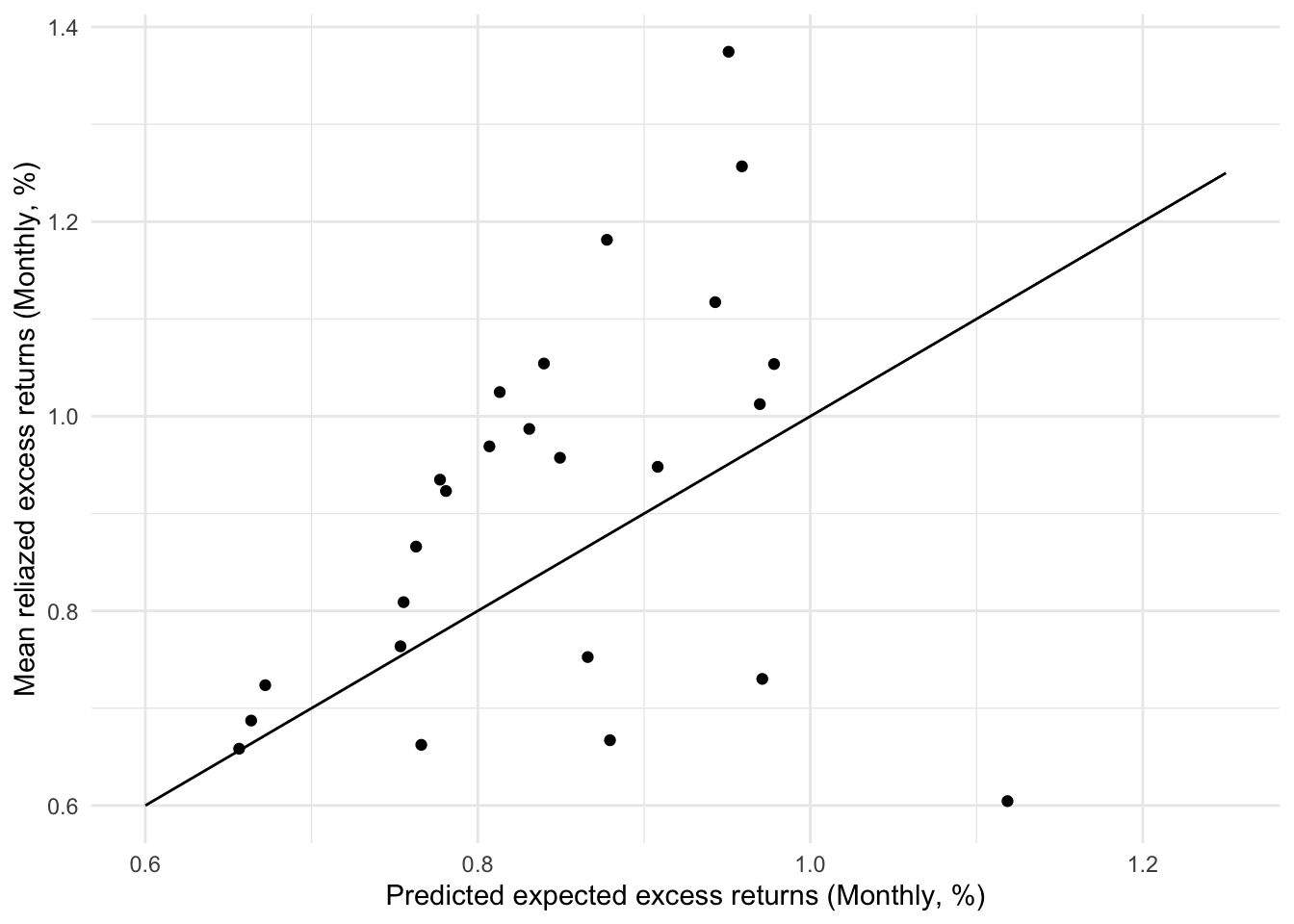

# t.test(alphas)
# mean(R2)

CAPM model assumes risk premium should be proportional to \(\beta\). In other words, the intercept \(\alpha\) here is expected to be 0. In all the linear regression models above, the slope (\(\beta\)) is statistically significant with 99.9% confidence level and all the intercepts are not that significant. The average difference between means and predictions is around 0.158%, which is very small. 8 out of the 25 differences are less the 0.1%. The average R squared of 25 regression models is 0.77. We can think that CAPM is already a good method to price the risk premium of the portfolios.

However, for some portfolios, the alphas are significant at 95% level. And by performing a t-test we can find that we cannot reject the null hypothesis (i.e., alpha = 0) at 90% confidence level. The plot above where the points are not located close enough to a line with slope at 1 implies CAPM model can be further improved to explain the realized excess returns by incorporating other factors.

4. Fama French 3 Factors

alphas = vector()
betas_mkt = vector()
betas_smb = vector()
betas_hml = vector()
preds_3factor = vector()
R2 = vector()
i=1
for (portfolio in colnames(data)[2:26]){
  model = lm(as.numeric(data[[portfolio]])-data[["RF"]] ~ data[["Mkt-RF"]]+data[["SMB"]]+data[["HML"]], na.action = na.omit)
  alphas[i] = model$coefficients[[1]]
  betas_mkt[i] = model$coefficients[[2]]
  betas_smb[i] = model$coefficients[[3]]
  betas_hml[i] = model$coefficients[[4]]
  R2[i] = summary(model)$r.squared
  preds_3factor[i] = mean(model$coefficients[2]*data[["Mkt-RF"]]+model$coefficients[3]*data[["SMB"]]+model$coefficients[4]*data[["HML"]],na.rm = T)
  i=i+1
}
ggplot()+
  geom_point(aes(x=preds_3factor,y=means))+
  geom_label(
    label=names
  )+
  labs(title="",
       x="Predicted expected excess returns",
       y="Mean reliazed excess returns")+
  geom_line(aes(x=c(0.6,1.4),y=c(0.6,1.4)))+
  theme_minimal()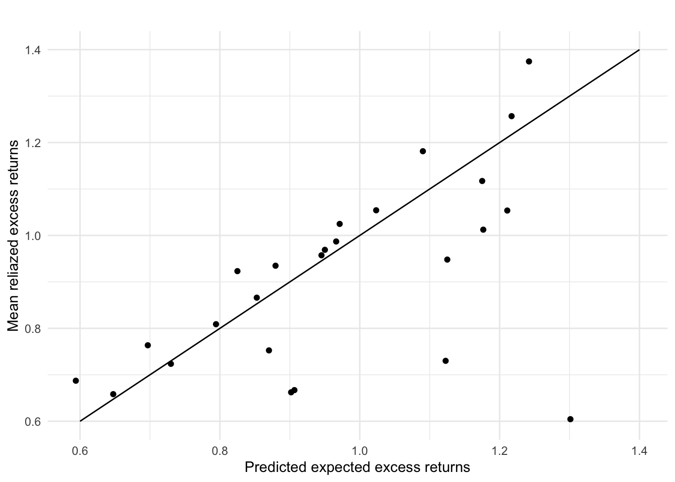

# t.test(alphas)
# mean(R2)

After adding SMB and HML factors, the average R squared has improved from 0.77 to 0.91. The difference between average predictions and average realized returns has decreased from 0.158% to 0.120%. 16 out of 25 portfolios have a difference smaller than 0.1%.

From the plot above we can observe that most points move closer to the line than previous one, indicating that Fama French 3 factors can better explain the excess return and price the risk premium of portfolios. With given beta, size and value factors, a portfolio can hardly over perform much over the predicted excess return.

However, we are still not able to reject the null hypothesis alpha = 0. Although they can on average explain 91% of the variance, the 3 factors still cannot capture all the factors affecting excess returns.

5. Cross-sectional data

Under this question, we will perform CAPM and Fama French 3 factors model on cross-sectional data after 1969-07 because data is only available after that month for health industry. We have 630 rows data with 165 portfolios so the regression can have statistical power.

# CAPM pricing
intercepts = vector()
betas_mkt = vector()
preds_all = vector()
means_all = vector()
data = data %>% drop_na()
i=1
for (portfolio in colnames(data)[-c(1,27:30)]){
  model = lm(as.numeric(data[[portfolio]])-data[["RF"]] ~ data[["Mkt-RF"]])
  
  intercepts[i] = model$coefficients[1]
  betas_mkt[i] = model$coefficients[2]
  means_all[i] = mean(as.numeric(data[[portfolio]])-data[["RF"]], na.rm = T)
  preds_all[i] = mean(rowSums(model$coefficients[2] * (data %>% select(`Mkt-RF`))),na.rm = T)
  i=i+1
}

ggplot()+
  geom_point(aes(x=preds_all,y=means_all))+
  geom_label(
    label=names
  )+
  labs(title="CAPM to all portfolios (Time-series regression)",
       x="Predicted expected excess returns",
       y="Mean reliazed excess returns")+
  geom_line(aes(x=c(0,1),y=c(0,1)))+
  theme_minimal()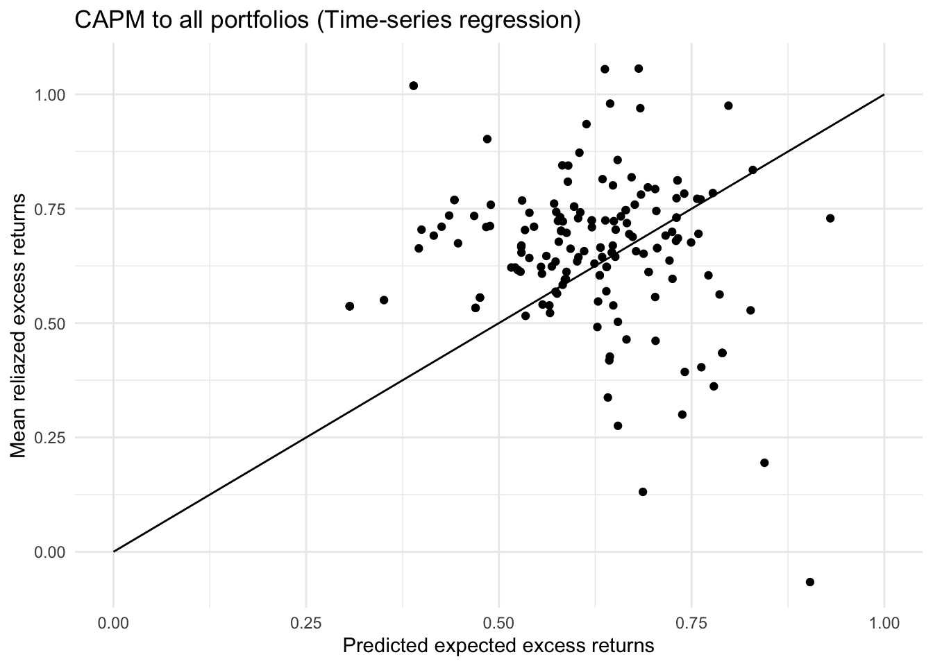

# cross-sectional regression
cross_section_intercepts = vector()
gamma_mkt = vector()
preds_cross_section = vector()
means_cross_section = vector()
cross_section_R2 = vector()

for (num in 1:nrow(data)){
  cross_sectional_data = data.frame(return = t(data[num,-c(1,27:30)]), 
                                  beta_mkt = betas_mkt)
  # modeling risk premium
  model = lm(return~beta_mkt,
             data=cross_sectional_data)
  cross_section_intercepts[num] = model$coefficients[1]
  gamma_mkt[num] = model$coefficients[2]
  means_cross_section[num] = mean(as.numeric(cross_sectional_data[["return"]]), na.rm = T)
  preds_cross_section[num] = mean(rowSums(model$coefficients[2] * (cross_sectional_data %>% select(beta_mkt))),na.rm = T)
  cross_section_R2[num] = summary(model)$r.squared
}

ggplot()+
  geom_point(aes(x=preds_cross_section,y=means_cross_section))+
  geom_label(
    label=names
  )+
  labs(title="CAPM to all portfolios (Cross-section)",
       x="Predicted expected excess returns",
       y="Mean reliazed excess returns")+
  geom_line(aes(x=c(-20,20),y=c(-20,20)))+
  theme_minimal()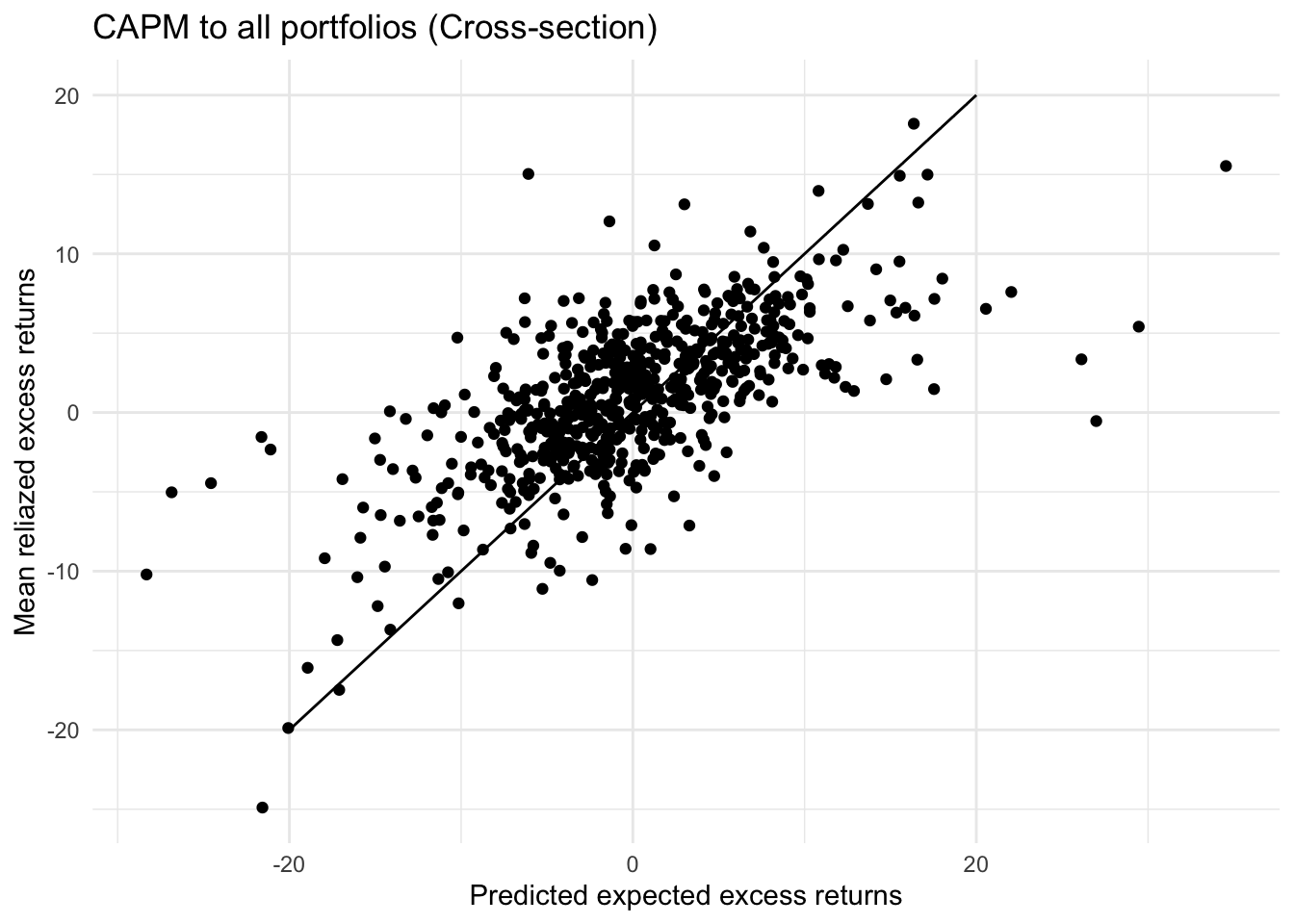

# t.test(intercepts)
# mean(cross_section_R2)

CAPM’s pricing ability on cross-sectional data is much less than that on time series data. The average R squared of the 630 regression models is only 0.1007. The alpha in the model is significantly different from 0 at 99.9% confidence level.

# Fama French pricing
intercepts = vector()
betas_mkt = vector()
betas_smb = vector()
betas_hml = vector()
preds_all = vector()
means_all = vector()
# For health industry, data is only available after 1969.07
data = data %>% drop_na()
i=1
for (portfolio in colnames(data)[-c(1,27:30)]){
  model = lm(as.numeric(data[[portfolio]])-data[["RF"]] ~ data[["Mkt-RF"]]+data[["SMB"]]+data[["HML"]])
  intercepts[i] = model$coefficients[1]
  betas_mkt[i] = model$coefficients[2]
  betas_smb[i] = model$coefficients[3]
  betas_hml[i] = model$coefficients[4]
  means_all[i] = mean(as.numeric(data[[portfolio]])-data[["RF"]], na.rm = T)
  preds_all[i] = mean(model$coefficients[2]*data[["Mkt-RF"]]+model$coefficients[3]*data[["SMB"]]+model$coefficients[4]*data[["HML"]],na.rm = T)
  i=i+1
}

ggplot()+
  geom_point(aes(x=preds_all,y=means_all))+
  geom_label(
    label=names
  )+
  labs(title="Fama French 3 factors to all portfolios (Time-series regression)",
       x="Predicted expected excess returns",
       y="Mean reliazed excess returns")+
  geom_line(aes(x=c(0,1),y=c(0,1)))+
  theme_minimal()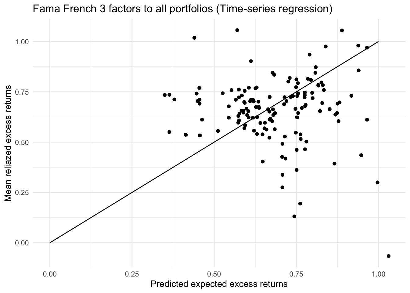

# cross-sectional regression
cross_section_intercepts = vector()
gamma_mkt = vector()
gamma_smb = vector()
gamma_hml = vector()
preds_cross_section = vector()
means_cross_section = vector()
cross_section_R2 = vector()
for (num in 1:nrow(data)){
  cross_sectional_data = data.frame(return = t(data[num,-c(1,27:30)]), 
                                    beta_mkt = betas_mkt,
                                    beta_smb = betas_smb,
                                    beta_hml = betas_hml)
  # modeling risk premium
  model = lm(return ~ beta_mkt + beta_smb + beta_hml,
             data=cross_sectional_data)
  cross_section_intercepts[num] = model$coefficients[1]
  gamma_mkt[num] = model$coefficients[2]
  gamma_smb[num] = model$coefficients[3]
  gamma_hml[num] = model$coefficients[4]
  means_cross_section[num] = mean(as.numeric(cross_sectional_data[["return"]]), na.rm = T)
  preds_cross_section[num] = mean(rowSums(model$coefficients[2:4] * (cross_sectional_data %>% select(beta_mkt,beta_smb,beta_hml))),na.rm = T)
  cross_section_R2[num] = summary(model)$r.squared
  
}
ggplot()+
  geom_point(aes(x=preds_cross_section,y=means_cross_section))+
  geom_label(
    label=names
  )+
  labs(title="Fama French 3 factors to all portfolios (Cross-section)",
       x="Predicted expected excess returns",
       y="Mean reliazed excess returns")+
  geom_line(aes(x=c(-20,20),y=c(-20,20)))+
  theme_minimal()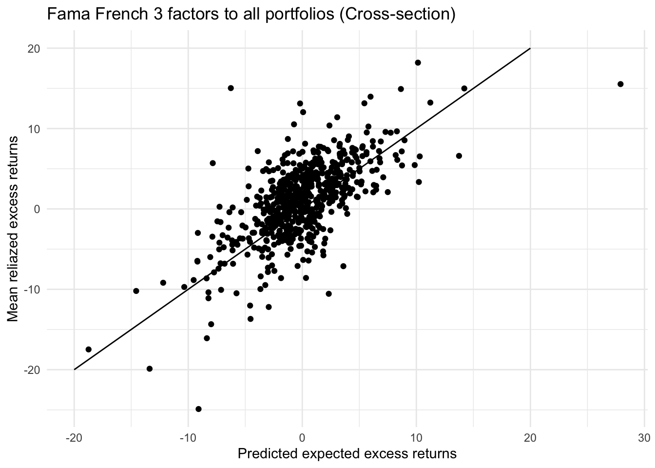

# t.test(cross_section_intercepts)
# mean(cross_section_R2)

Fama French 3 factors model can price the risk premium on cross-sectional data better than CAPM. The points on the plot seem more linear here but much more volatile than those on time-series data of single portfolio. However, the average R squared has increased from 0.1007 to 0.1996, but it’s still a very small proportion of total variance. The intercept is significantly different from 0. Therefore, based on the factors estimated on data from 1969-07 to 2021-12, the pricing ability Fama French 3 factors model is far weaker than that on time series data.

6. Momentum factor

Since we have seen that the Fama French 3 factors model can be improved, momentum factor will be introduced here to enrich the model. First we need to calculate momentum of all the stocks in the market. Then we can set up a momentum factor by applying Fama and French approach, which means to set up a portfolio which long $1 of large momentum and short \$1 of small (negative) momentum. As in (Jegadeesh & Titman, 2011), the profits of momentum strategy can be partly explained by value-weighted index over the previous 36 months and Strivers and Sun (2010) RD variable. We may adjust the momentum factor to make it more independent from other factors. This portfolio also needs to be rebalanced periodically to allow migrations between momentum categories. After obtaining the returns on momentum factor, we can empirically test the new model by running time-series regression and cross-ssection regression models using 4-factor model to see whether the new model can explain more variance and lower the unexplained alphas plus residuals than the previous Fama French 3 factors model.

Comments on statements

– The Fama-French three factor model is as good as it gets. Hence, we should always use this model.

There is no silver bullets to explain security returns. Although Fama French 3 factor model can explain on average 91% of the variance on time series data, it’s not the perfect model and the behavior of investors can even be different in different markets at different time, which makes it impossible to say this model can fit in all situations with equally strong pricing ability. So far researchers have explored and tested a lot of factors in many markets. We can either refer to their results or implement our own insights of the financial market to develop a better model, rather than limit ourselves to Fama French 3 factor model. The Morningstar’s benchmarks can also be very good practical choice.

– As the Fama-French three factor model performs empirically superior to the CAPM, we might as well forget about CAPM entirely.

CAPM as a simple and static but powerful model is the basis of Fama French 3 factor model and lots of variations to explain returns. It is already able to effectively predict returns of securities. When adding SMB and HML variable cannot significantly increase the prediction power, CAPM can be a better model possibly with other factors.

– Empirically, the best factor model has three factors.

We have observed that 3 factor model is better than CAPM model on both time series data and cross sectional data. But we cannot reach a conclusion about which model is the best. Since our empirical tests are only performed with 3 factors at most on US market data from 1969-07 to 2021-12. It’s not sufficient to generalize the result to such a conclusion.

– Empirically, the best factor model has five factors.

In this assignment, we didn’t performed empirical tests of 5 factor model. Even if we have done it, it’s nearly impossible to reach a conclusion about which regression model is the best. Since the performance of model largely depends on the market behavior, even best model will deteriorate. In addition, the pricing model doesn’t follow a “the more, the better” rule. More factors cannot guarantee better model performance.

– The validity of CAPM cannot be tested empirically.

Although Robert Haugen (1999) once said “CAPM also makes use of what is called a”definitional identity.” This is something that is automatically true, simply because of the way things have been defined.”, there are a lot of researchers performing empirical tests on CAPM and verifying its validity by applying the method proposed in Fama and Macbeth (1973). Eugene and Kenneth (2005) points out the difficulty of testing CAPM empirically is due to the lack of theoretical or empirical clarity on what constitutes the market portfolio. What the empirical results test is actually the efficiency of market portfolio proxy instead of the validity of CAPM.

Calculating log returns

hpr = read_xlsx("PS1_Daily.xlsx", sheet = 1, skip = 1)
prices = read_xlsx("PS1_Daily.xlsx", sheet = 2, skip = 1)
for (stock in colnames(prices)[2:8]){
  prices[[paste(stock,"log",sep = "_")]] = log(prices[[stock]]/lag(prices[[stock]]))
}

ACF plots

ggAcf(prices$SPINDX_log^2)+ggAcf(abs(prices$SPINDX_log))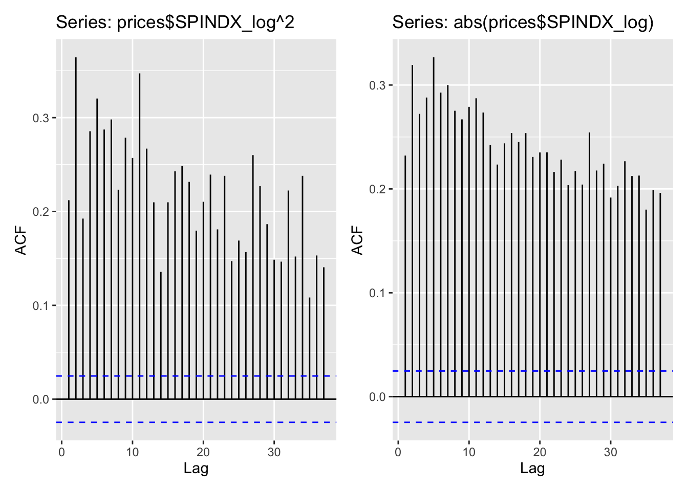

Squared and absolute returns are statistically significantly (far over the blue dashed line) autocorrelated. The maximum autocorrelation coefficient reaches over 0.35 for squared returns and over 0.32 for absolute returns. Although it’s not very strong autocorrelation, we can conclude that they are predictable with previous data. However, for both series of data, the most recent data point is not most related with current one. For squared returns, the data point of lag 2 day can be the best predictor. For absolute returns, it becomes lag 5.

Moving average model - Microsoft

# W=10
vol_10 = c(NaN)
for (i in 2:nrow(prices)+1){
  vol_10 = append(vol_10, mean(prices$MSFT_log[max(0,i-11):(i-1)]^2,na.rm = T))
}

# W=20
vol_20 = c(NaN)
for (i in 2:nrow(prices)){
  vol_20 = append(vol_20, mean(prices$MSFT_log[max(0,i-21):(i-1)]^2,na.rm = T))
}
ts.plot(vol_10, main = "MA model on Microsoft (time window = 10d)")

ts.plot(vol_20, main = "MA model on Microsoft (time window = 20d)")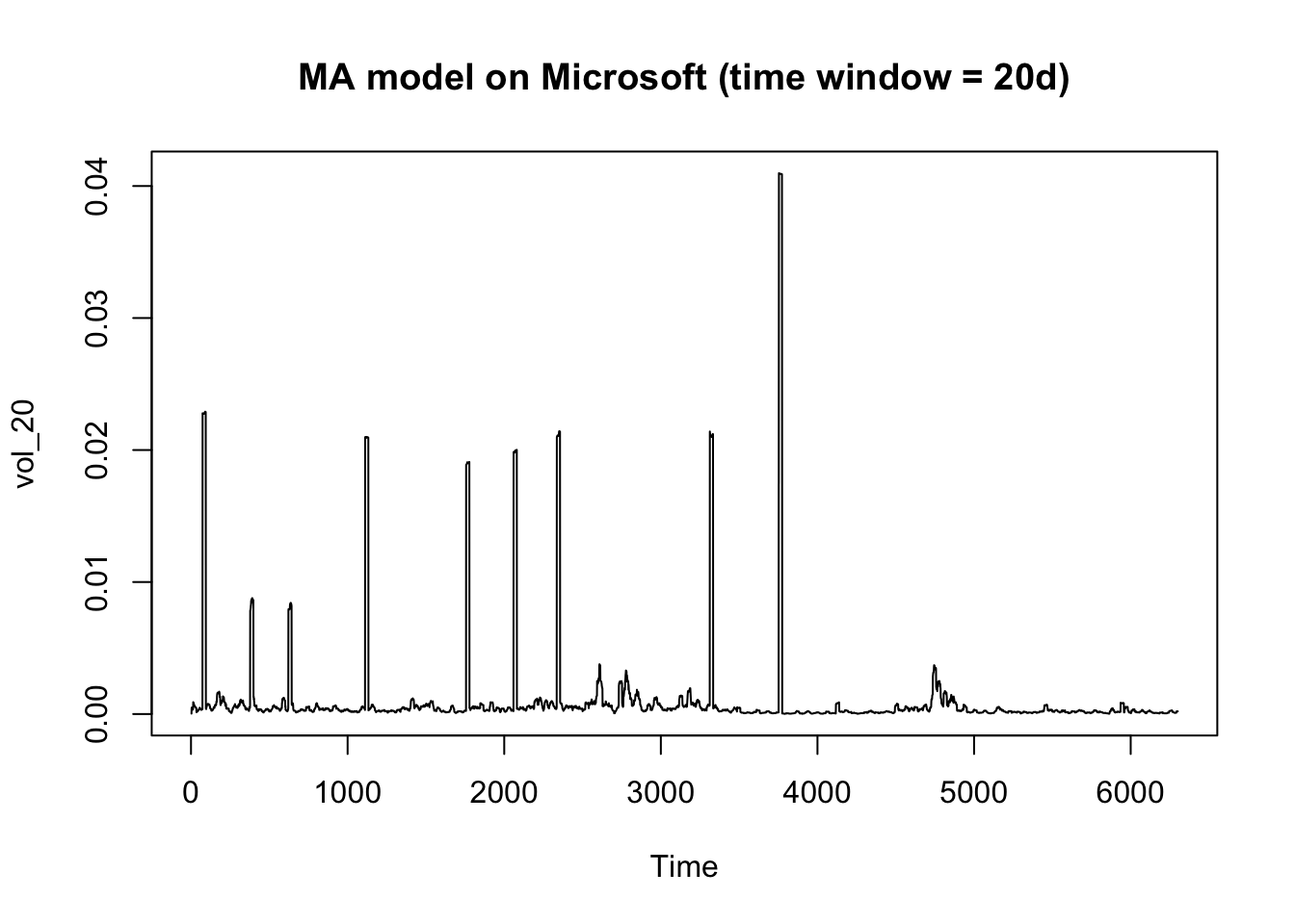

Modern portfolio theory summarize investment properties of securities by their expected returns and volatility. With given expected return, it tries to minimize the risk, while with given volatility, it tries to maximize the expected return.

However, in this question we have figured out the relationship between return and volatility. If several series data of returns are available, we are able to not only make a decision of portfolio struture based on historical data, but also predict the volatility of the next time period and rebalance the portfolio in time to minimize the future volatility and avoid the risk.

Moving average model - S&P500

# W=10
vol_10 = c(NaN)
for (i in 2:nrow(prices)+1){
  vol_10 = append(vol_10, mean(prices$SPINDX_log[max(0,i-11):(i-1)]^2,na.rm = T))
}

# W=20
vol_20 = c(NaN)
for (i in 2:nrow(prices)){
  vol_20 = append(vol_20, mean(prices$SPINDX_log[max(0,i-21):(i-1)]^2,na.rm = T))
}
ts.plot(vol_10, main = "MA model on S&P 500 (time window = 10d)")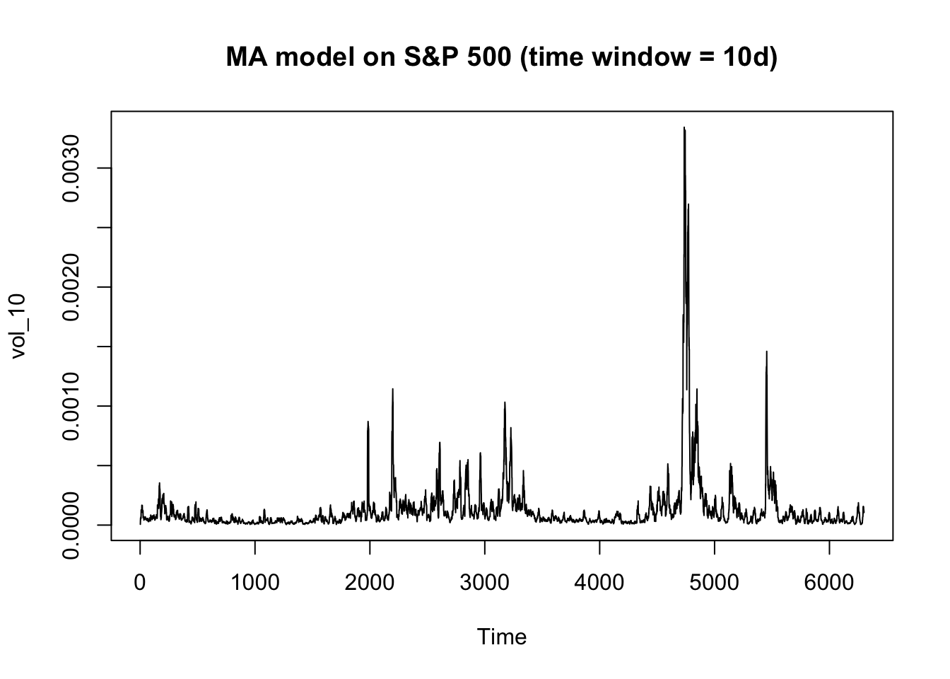

ts.plot(vol_20, main = "MA model on S&P 500 (time window = 20d)")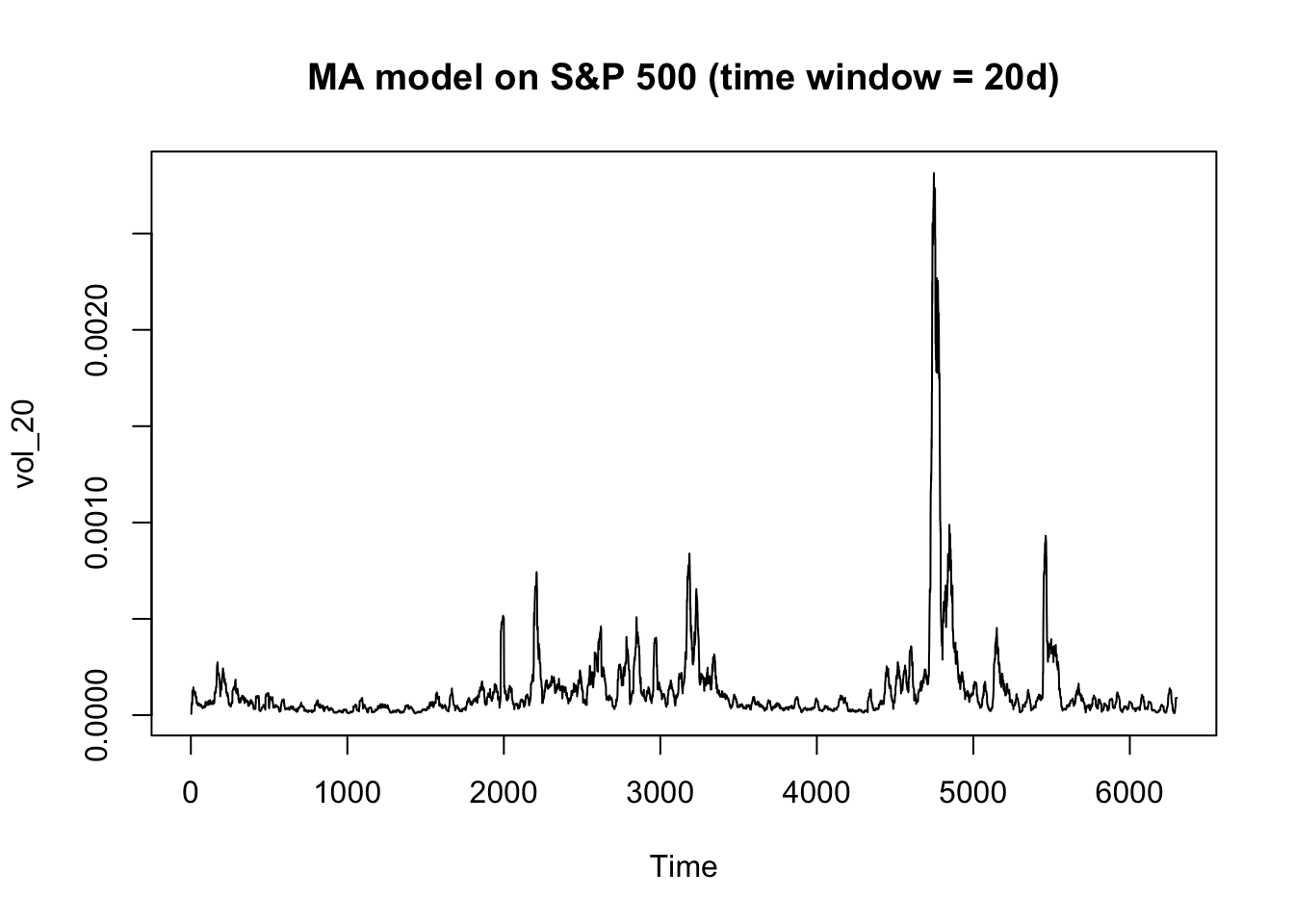

The squared return of S&P 500 is much less volatile than that of Microsoft. The plot of a moving average model with 10-day time window is clear enough to observe the general trend for S&P 500. But there are many abnormal spikes in the Microsoft plot, indicating the volatility of Microsoft is less predictable so that it’s riskier to invest in the stock than the index.

EWMA - S&P500

Assumption about \(\sigma_0^2\): a sensible starting value could be the squared log return of the first day. This value should be very close to the actual value of that day because of the significant autocorrelation of the squared log returns. And this calculation is close to MA method in the initial stage. Other values are not so sensible such as, 0 will make the following values unnecessarily lower because of missing the whole lambda*sigma^2 item in the formula, any too large heuristic values will lead to a much larger averaged value in the following days to eliminate the effects of initial value. The variance of the series can be a good estimation as well, but the information should not be available on the first day of the series. Therefore, in the following analysis of the delay factor, the starting point will be set at the squared value of the first log return.

lambda = 0.5
vol_ewma_50 = c(0,prices$SPINDX_log[2]^2) # it's the squared value of the first log return
for (i in 3:nrow(prices)){
  vol_ewma_50[i] = (1-lambda) * prices$SPINDX_log[i-1]^2 + lambda* vol_ewma_50[i-1]
}

lambda = 0.75
vol_ewma_75 = c(0,prices$SPINDX_log[2]^2)
for (i in 3:nrow(prices)){
  vol_ewma_75[i] = (1-lambda) * prices$SPINDX_log[i-1]^2 + lambda* vol_ewma_75[i-1]
}

lambda = 0.94
vol_ewma_94 = c(0,prices$SPINDX_log[2]^2)
for (i in 3:nrow(prices)){
  vol_ewma_94[i] = (1-lambda) * prices$SPINDX_log[i-1]^2 + lambda* vol_ewma_94[i-1]
}


ts.plot(vol_ewma_50)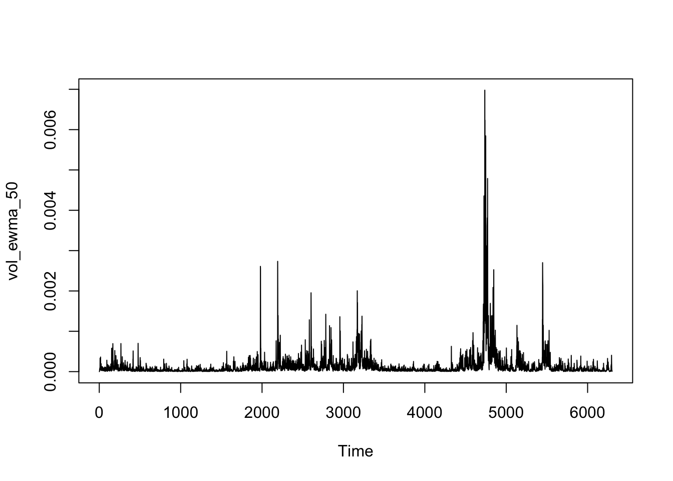

ts.plot(vol_ewma_75)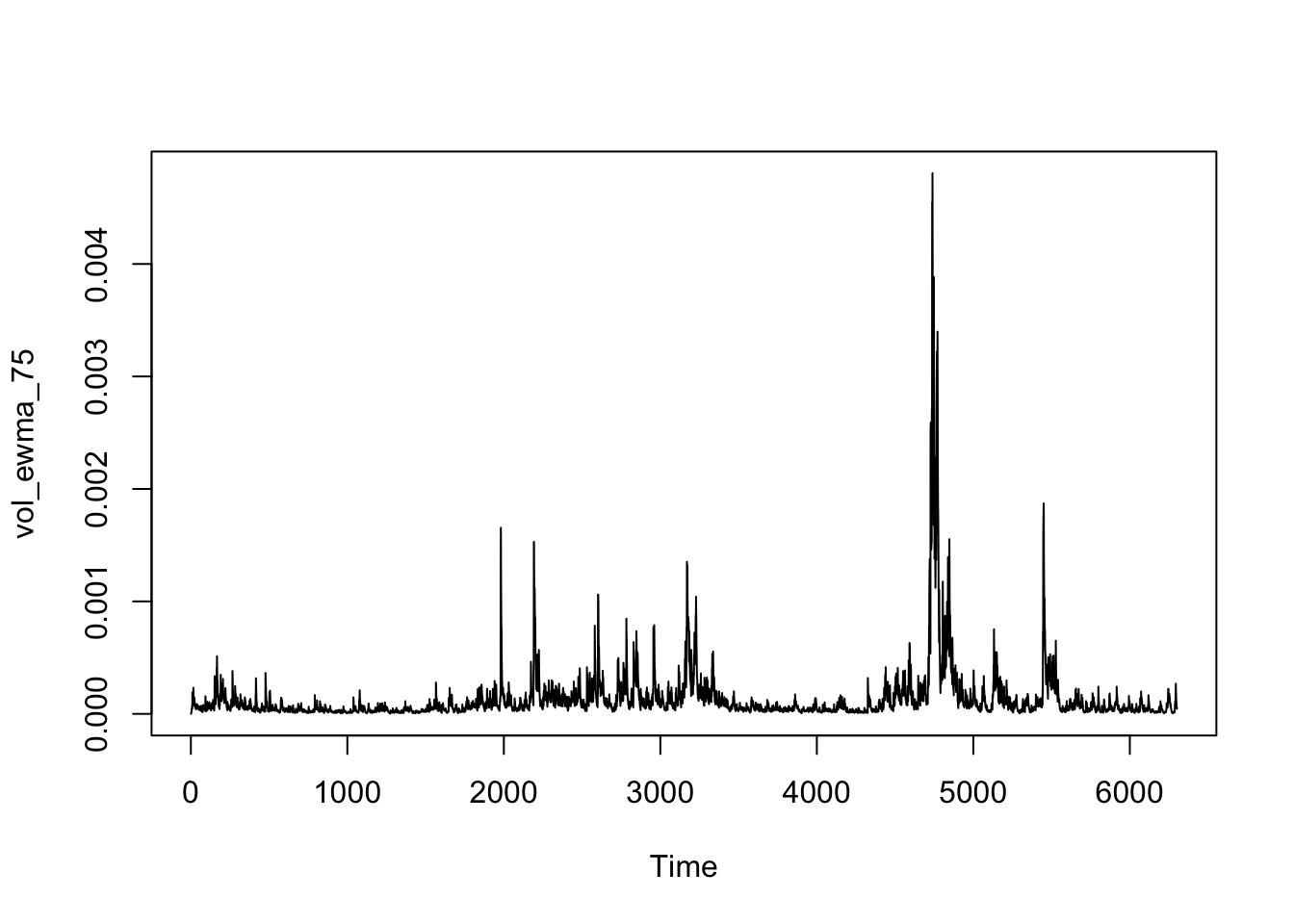

ts.plot(vol_ewma_94)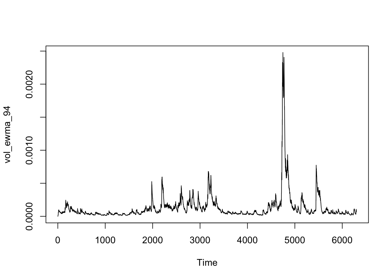

As the delay factor, a higher lambda will lead the model to focus more on recent data points and less on the previous average, which makes the data points more volatile. Since daily data is very volatile, so a higher lambda should be applied to smooth the daily volatility. 0.94 is a relevantly good choice to make the plot reflect the trend of daily volatility as the third plot shows above.

References

[1] Fama, E. F., & MacBeth, J. D. (1973). Risk, Return, and Equilibrium: Empirical Tests. Journal of Political Economy, 81(3), 607–636. http://www.jstor.org/stable/1831028 [2] Fama, E. F., & French, K. R. (1992). The cross‐section of expected stock returns. the Journal of Finance, 47(2), 427-465. [3] How to do Fama French (1993) cross sectional regressions? A few questions. https://quant.stackexchange.com/questions/55070/how-to-do-fama-french-1993-cross-sectional-regressions-a-few-questions.