Voting in the UN General Assembly

Data

The unvotes package provides three datasets we can work with: un_roll_calls, un_roll_call_issues, and un_votes. Each of these datasets contains a variable called rcid, the roll call id, which can be used as a unique identifier to join them with each other.

• The un_votes dataset provides information on the voting history of the United Nations General Assembly. It contains one row for each country-vote pair.

un_votes

## # A tibble: 869,937 × 4
##     rcid country            country_code vote 
##    <dbl> <chr>              <chr>        <fct>
##  1     3 United States      US           yes  
##  2     3 Canada             CA           no   
##  3     3 Cuba               CU           yes  
##  4     3 Haiti              HT           yes  
##  5     3 Dominican Republic DO           yes  
##  6     3 Mexico             MX           yes  
##  7     3 Guatemala          GT           yes  
##  8     3 Honduras           HN           yes  
##  9     3 El Salvador        SV           yes  
## 10     3 Nicaragua          NI           yes  
## # … with 869,927 more rows

• The un_roll_calls dataset contains information on each roll call vote of the United Nations General Assembly.

un_roll_calls

## # A tibble: 6,202 × 9
##     rcid session importantvote date       unres   amend  para short        descr
##    <int>   <dbl>         <int> <date>     <chr>   <int> <int> <chr>        <chr>
##  1     3       1             0 1946-01-01 R/1/66      1     0 AMENDMENTS,… "TO …
##  2     4       1             0 1946-01-02 R/1/79      0     0 SECURITY CO… "TO …
##  3     5       1             0 1946-01-04 R/1/98      0     0 VOTING PROC… "TO …
##  4     6       1             0 1946-01-04 R/1/107     0     0 DECLARATION… "TO …
##  5     7       1             0 1946-01-02 R/1/295     1     0 GENERAL ASS… "TO …
##  6     8       1             0 1946-01-05 R/1/297     1     0 ECOSOC POWE… "TO …
##  7     9       1             0 1946-02-05 R/1/329     0     0 POST-WAR RE… "TO …
##  8    10       1             0 1946-02-05 R/1/361     1     1 U.N. MEMBER… "TO …
##  9    11       1             0 1946-02-05 R/1/376     0     0 TRUSTEESHIP… "TO …
## 10    12       1             0 1946-02-06 R/1/394     1     1 COUNCIL MEM… "TO …
## # … with 6,192 more rows

• The un_roll_call_issues dataset contains (topic) classifications of roll call votes of the United Nations General Assembly. Many votes had no topic, and some have more than one. In our dataset, there are six topics and

un_roll_call_issues

## # A tibble: 5,745 × 3
##     rcid short_name issue               
##    <int> <chr>      <fct>               
##  1    77 me         Palestinian conflict
##  2  9001 me         Palestinian conflict
##  3  9002 me         Palestinian conflict
##  4  9003 me         Palestinian conflict
##  5  9004 me         Palestinian conflict
##  6  9005 me         Palestinian conflict
##  7  9006 me         Palestinian conflict
##  8   128 me         Palestinian conflict
##  9   129 me         Palestinian conflict
## 10   130 me         Palestinian conflict
## # … with 5,735 more rows

Analysis

First, let’s take a look at how often each country voted “Yes” on a resolution in each year. We’ll visualize the results, so let’s pick a few countries of interest first,

country_list <- c("United States of America", "China", 
                  "United Kingdom of Great Britain and Northern Ireland", "India")

and focus our analysis on them.

un_votes %>%
  filter(country %in% country_list) %>%
  inner_join(un_roll_calls, by = "rcid") %>%
  group_by(year = year(date), country) %>%
  summarize(
    votes = n(),
    percent_yes = mean(vote == "yes")
    ) %>%
  ggplot(mapping = aes(x = year, y = percent_yes, color = country)) +
    geom_line() +
    labs(
      title = "Percentage of 'Yes' votes in the UN General Assembly",
      subtitle = "1946 to 2015",
      y = "% Yes",
      x = "Year",
      color = "Country"
    )+
  theme_bw()

## `summarise()` has grouped output by 'year'. You can override using the
## `.groups` argument.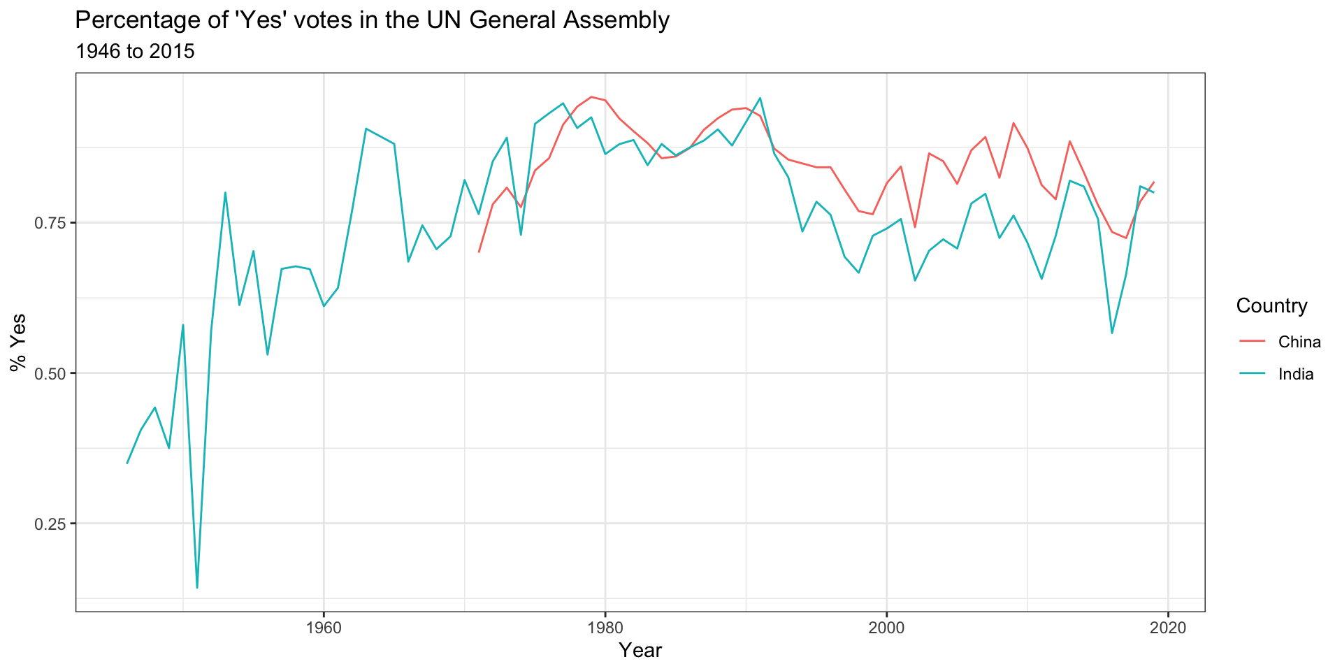

Next, let’s create a visualization that displays how the voting record of the United States changed over time on a variety of issues, and compares it to another country. The other country we’ll display is India.

un_votes %>%
  filter(country %in% c("United States of America", "India")) %>%
  inner_join(un_roll_calls, by = "rcid") %>%
  inner_join(un_roll_call_issues, by = "rcid") %>%
  group_by(country, year = year(date), issue) %>%
  summarize(
    votes = n(),
    percent_yes = mean(vote == "yes")
    ) %>%
  filter(votes > 5) %>%  # only use records where there are more than 5 votes
  ggplot(mapping = aes(x = year, y = percent_yes, color = country)) +
    geom_point() +
    geom_smooth(method = "loess", se = FALSE) +
    facet_wrap(~ issue) +
    labs(
      title = "Percentage of 'Yes' votes in the UN General Assembly",
      subtitle = "1946 to 2015",
      y = "% Yes",
      x = "Year",
      color = "Country"
    )+
  theme_bw()

## `summarise()` has grouped output by 'country', 'year'. You can override using
## the `.groups` argument.
## `geom_smooth()` using formula 'y ~ x'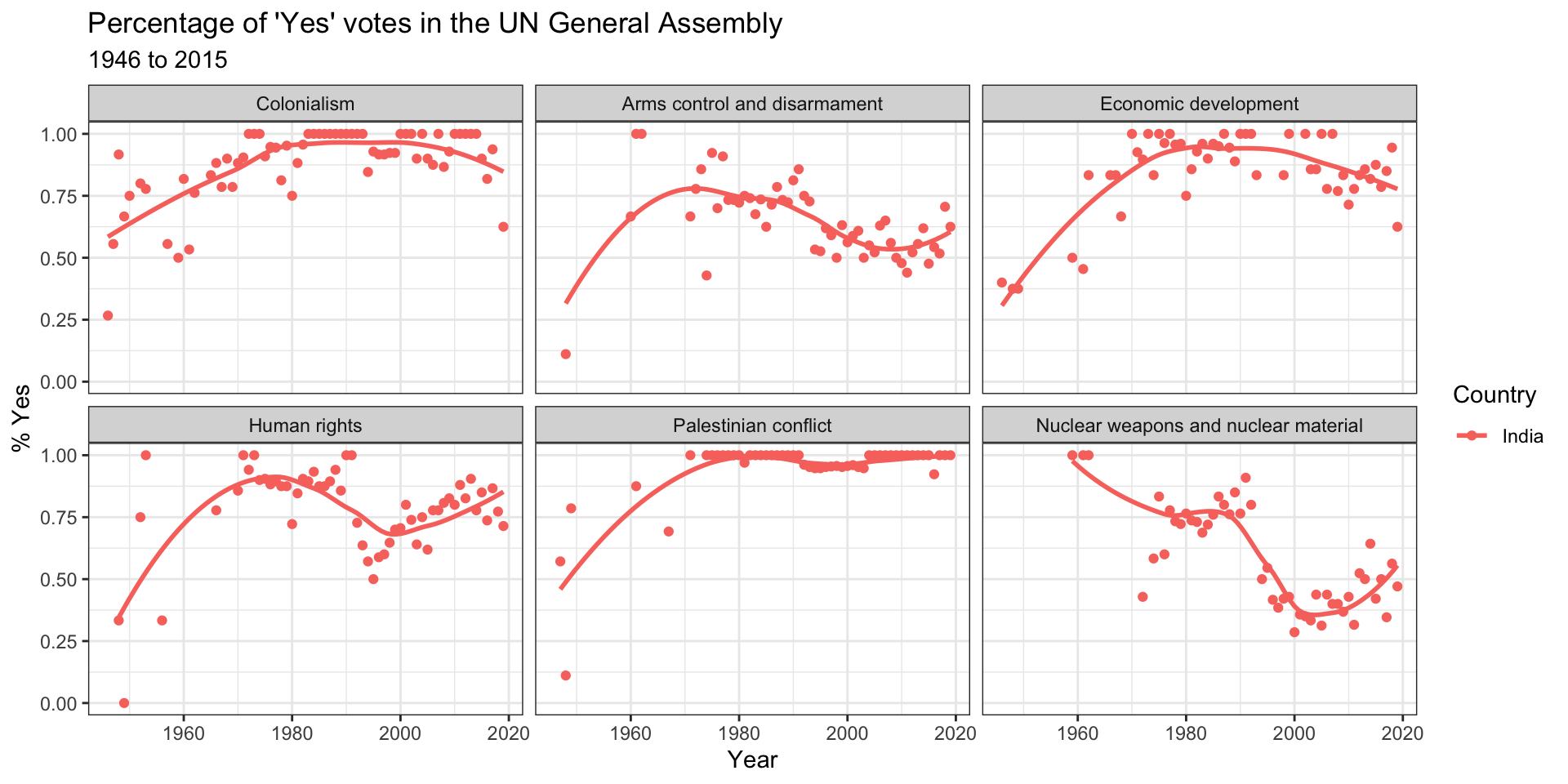

We can easily change which countries are being plotted by changing which countries the code above filters for. Note that the country name should be spelled and capitalized exactly the same way as it appears in the data. See the Appendix for a list of the countries in the data.

References

1. David Robinson (2017). unvotes: United Nations General Assembly Voting Data. R package version 0.2.0. https://CRAN.R-project.org/package=unvotes.
2. Erik Voeten “Data and Analyses of Voting in the UN General Assembly” Routledge Handbook of International Organization, edited by Bob Reinalda (published May 27, 2013).
3. Much of the analysis has been modeled on the examples presented in the unvotes package vignette.

Appendix

Below is a list of countries in the dataset:

un_votes %>% 
  select(country) %>%
  arrange(country) %>% 
  distinct() %>%
  datatable()