Many Regressions
Publish date: Nov 14, 2021Tags: Stats
library(broom)
library(forcats)
yearMin <- 1952
many_models <- gapminder %>%
  # create a dataframe containing a separate dataframe for each country
  group_by(country,continent) %>%

  # nesting creates a list-column of data frames;
  # we will use the list to fit a regression model for every country
  nest()  %>%

  # Run a simple regression model for every country in the dataframe
  mutate(simple_model = data %>%
           map(~lm(lifeExp ~ I(year - yearMin), data = .))) %>%

  # extract coefficients and model details with broom::tidy
  mutate(coefs = simple_model %>% map(~ tidy(., conf.int = TRUE)),
         details = simple_model %>% map(glance)) %>%
  ungroup()

head(many_models, 10)
## # A tibble: 10 × 6
## country continent data simple_model coefs details
## <fct> <fct> <list> <list> <list> <list>
## 1 Afghanistan Asia <tibble [12 × 4]> <lm> <tibble> <tibble>
## 2 Albania Europe <tibble [12 × 4]> <lm> <tibble> <tibble>
## 3 Algeria Africa <tibble [12 × 4]> <lm> <tibble> <tibble>
## 4 Angola Africa <tibble [12 × 4]> <lm> <tibble> <tibble>
## 5 Argentina Americas <tibble [12 × 4]> <lm> <tibble> <tibble>
## 6 Australia Oceania <tibble [12 × 4]> <lm> <tibble> <tibble>
## 7 Austria Europe <tibble [12 × 4]> <lm> <tibble> <tibble>
## 8 Bahrain Asia <tibble [12 × 4]> <lm> <tibble> <tibble>
## 9 Bangladesh Asia <tibble [12 × 4]> <lm> <tibble> <tibble>
## 10 Belgium Europe <tibble [12 × 4]> <lm> <tibble> <tibble>The resulting dataframe many_models contains for every country the country data, the regression model simple_model, the model coefficients coefs, as well as all the regression details. As discussed earlier, the intercept is the predicted life expectancy in 1952 and the slope is the average yearly improvement in life expectancy.
We will take our many_models dataframe, unnest the coefs and extract the interecept and slope for each country.
intercepts <-
  many_models %>%
  # Unnesting flattens a list-column of data frames back into regular columns
  unnest(coefs) %>%
  filter(term == "(Intercept)") %>%
  arrange(estimate) %>%
  mutate(country = fct_inorder(country)) %>%
  select(country, continent, estimate, std.error, conf.low, conf.high)

# let us look at the first 20 intercepts, or life expectancy in 1952
head(intercepts,20)
## # A tibble: 20 × 6
## country continent estimate std.error conf.low conf.high
## <fct> <fct> <dbl> <dbl> <dbl> <dbl>
## 1 Gambia Africa 28.4 0.623 27.0 29.8
## 2 Afghanistan Asia 29.9 0.664 28.4 31.4
## 3 Yemen, Rep. Asia 30.1 0.861 28.2 32.0
## 4 Sierra Leone Africa 30.9 0.448 29.9 31.9
## 5 Guinea Africa 31.6 0.649 30.1 33.0
## 6 Guinea-Bissau Africa 31.7 0.349 31.0 32.5
## 7 Angola Africa 32.1 0.764 30.4 33.8
## 8 Mali Africa 33.1 0.262 32.5 33.6
## 9 Mozambique Africa 34.2 1.24 31.4 37.0
## 10 Equatorial Guinea Africa 34.4 0.178 34.0 34.8
## 11 Nepal Asia 34.4 0.502 33.3 35.5
## 12 Somalia Africa 34.7 1.01 32.4 36.9
## 13 Burkina Faso Africa 34.7 1.11 32.2 37.2
## 14 Niger Africa 35.2 1.19 32.5 37.8
## 15 Eritrea Africa 35.7 0.813 33.9 37.5
## 16 Ethiopia Africa 36.0 0.569 34.8 37.3
## 17 Bangladesh Asia 36.1 0.530 35.0 37.3
## 18 Djibouti Africa 36.3 0.612 34.9 37.6
## 19 Madagascar Africa 36.7 0.304 36.0 37.3
## 20 Senegal Africa 36.7 0.506 35.6 37.9slopes <- many_models %>%
unnest(coefs) %>%
filter(term == "I(year - yearMin)") %>%
arrange(estimate) %>%
mutate(country = fct_inorder(country)) %>%
select(country, continent, estimate, std.error, conf.low, conf.high)
# let us look at the first 20 slopes, or average improvement in life exepctancy per year
head(slopes,20)## # A tibble: 20 × 6
## country continent estimate std.error conf.low conf.high
## <fct> <fct> <dbl> <dbl> <dbl> <dbl>
## 1 Zimbabwe Africa -0.0930 0.121 -0.362 0.175
## 2 Zambia Africa -0.0604 0.0757 -0.229 0.108
## 3 Rwanda Africa -0.0458 0.110 -0.290 0.199
## 4 Botswana Africa 0.0607 0.102 -0.167 0.288
## 5 Congo, Dem. Rep. Africa 0.0939 0.0406 0.00338 0.184
## 6 Swaziland Africa 0.0951 0.111 -0.153 0.343
## 7 Lesotho Africa 0.0956 0.0992 -0.126 0.317
## 8 Liberia Africa 0.0960 0.0297 0.0299 0.162
## 9 Denmark Europe 0.121 0.00667 0.106 0.136
## 10 Uganda Africa 0.122 0.0533 0.00280 0.240
## 11 Hungary Europe 0.124 0.0199 0.0794 0.168
## 12 Cote d'Ivoire Africa 0.131 0.0657 -0.0157 0.277
## 13 Norway Europe 0.132 0.00819 0.114 0.150
## 14 Slovak Republic Europe 0.134 0.0217 0.0856 0.182
## 15 Netherlands Europe 0.137 0.00582 0.124 0.150
## 16 Czech Republic Europe 0.145 0.0138 0.114 0.176
## 17 Bulgaria Europe 0.146 0.0420 0.0522 0.239
## 18 Burundi Africa 0.154 0.0269 0.0941 0.214
## 19 Paraguay Americas 0.157 0.00655 0.143 0.172
## 20 Romania Europe 0.157 0.0245 0.103 0.212We can plot the estimates for the intercept and the slope for all countries, faceted by continent.
  ggplot(data = intercepts,
         aes(x = country, y = estimate, fill=continent))+
  geom_col()+
  coord_flip()+
  theme_minimal(6)+
  facet_wrap(~continent, scales="free")+
  labs(title = 'Life expectancy in 1952',
       caption = 'Source: Gapminder package',
       x = "") +
  theme(legend.position="none")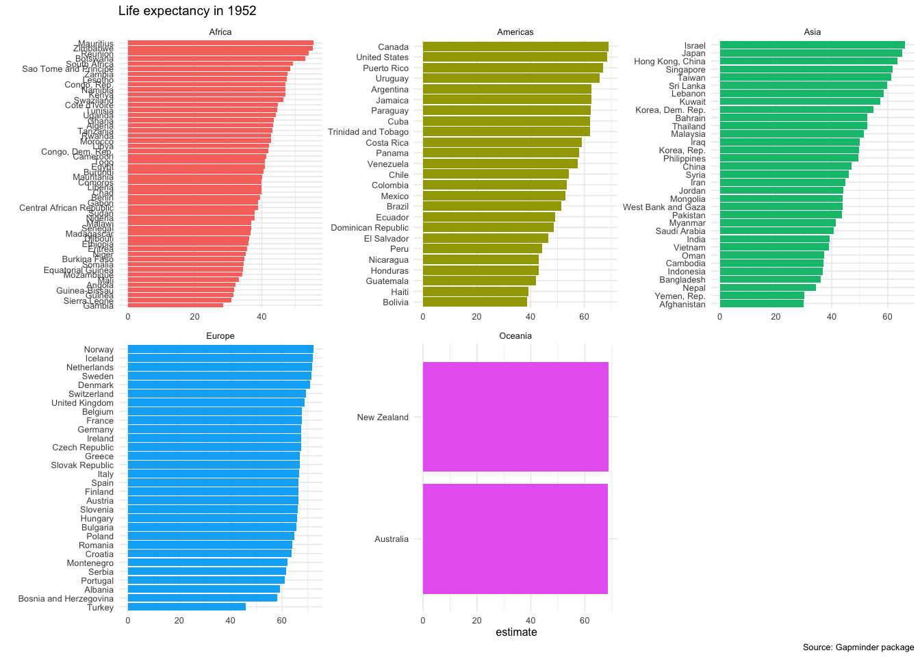
  ggplot(data = slopes,
         aes(x = country, y = estimate, fill = continent))+
  geom_col()+
  coord_flip()+
  theme_minimal(6)+
  facet_wrap(~continent, scales="free")+
  labs(title = 'Average yearly improvement in life expectancy, 1952-2007',
       caption = 'Source: Gapminder package',
       x = "") +
  theme(legend.position="none")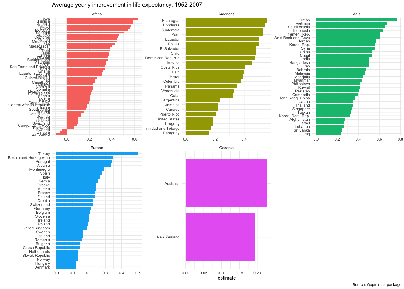
Finally, as in every regression model, the slopes are estimates for the yearly improvement in life expectancy. If we wanted to, we can plot the confidence interval for each country’s improvement.
ggplot(data = slopes,
       aes(x = country, y = estimate, colour = continent))+
  geom_pointrange(aes(ymin = conf.low, ymax = conf.high))+
  coord_flip()+
  theme_minimal(6)+
  facet_wrap(~continent, scales="free")+
  labs(title = 'Average yearly improvement in life expectancy, 1952-2007',
       caption = 'Source: Gapminder package',
       x = "") +
  theme(legend.position="none")